up
german
"The problem of understanding behavior is the problem of understanding the total action of the nervous system, and vice versa"
Donald Olding Hebb (1949)
The Second Informatics
Overview about Properties of Interference Networks
Gerd Heinz
The page provides an overview* of ways to process information with slow-flowing pulses (interference integrals and interference networks). They differ fundamentally from known digital circuits, which is why we want to call them a "Second Informatics".
Note
The circuits shown here as interference networks are not electrical networks, but rather nervous networks with extremely low conduction velocities. All lines are delay lines. The electrical node abstraction of a line is not valid here. Overcoming any distance takes a lot of time!
What peculiarities of the nervous system led to the birth of interference networks?
We find mirror-image maps everywhere in the nervous system. Body projections in the homunculus are mirrored, see
Chapter 8 on the biomodels page.
Such mirror-image maps are not known from artificial neural networks (ANN).
Weights in ANN are controlled by the PC algorithm via a virtually infinitely fast action at a distance.
Time also progresses in discrete steps (clocks).
Both assumptions do not apply in nerve networks, however. Their information transfer is very slow.
Because clock lines would also be much too slow, nerve networks do not have a synchronizing clock.
 How is it possible, that a two-millimeter fruit fly (Drosophilidae), whose cortex is perhaps a tenths of a millimeter in size, can orient itself in space, control its wings and also find food? Can we ever move into this area with our microelectronics and computer science? Or does nature have much more efficient options than we do?
When we think about information processing on wires, including nervous processing, we first have to distinguish between analog and binary processing.
With analog processing, floating values are transmitted. These can be voltage values, as measured by a voltmeter or oscilloscope, or potentials that appear in EEG or EKG.
With binary or digital processing, however, only the values zero or one, corresponding to LOW or HIGH, are transmitted. This type of transmission offers the advantage of maximum immunity against disturbances, so binary processing is very dominant in the field of technology.
We distinguish between two basic forms of binary processing:
-
A transmission that is tied to a time (clock). These can be clocks, baud rates or frequencies that indicate the validity of a signal to the receiver.
-
Nerves, on the other hand, have a very low conduction speed, so clocks, baud rates or cycles are unknown. Instead, we find pulse-shaped signals everywhere.
The basic question for understanding the nervous system is the question of the way of clock-free processing of pulse-shaped signals, that flow very slowly through nerves.
How do they work? What do we know about this previously completely unknown field of this second informatics? We enter the field of Interference Networks (IN).
When a nerve cell is stimulated, it generally responds with a brief impulse. If it is more strongly stimulated, it pulses faster, there is an increase in pulse frequency. The pulse amplitude always remains constant. Excitation is coded as pulse rate.
We find this basic form of signaling in the nervous system in all known species. Adrian received the Nobel Prize in 1932 for his fundamental contribution to the research of the function of nerve impulse mechanism.
For detailed investigations of nervous pulse parameters, Hodgkin, Huxley and Eccles followed with the Nobel Prize for Medicine in 1963, while Erlanger and Gasser systematically examined the conduction velocities of various nerves. John Eccles noticed about the relationship between the fiber diameter of the nerve and the conduction velocity:
"The conduction speed (in m/s) is approximately proportional to the fiber diameter (in µm), whereby the ratio for mammalian nerves is about 6:1; ie a large nerve fiber of 20 µm diameter ... would conduct impulses at about 120 meters per second."
(Quote from John Eccles (1973): The Understanding of the Brain, ch.1, p.50)
The author noticed in 1992, that a short pulse duration t together with a slow conduction velocity v produces geometrically such extremely short pulse lengths s, that they do not fit with our computer science. For details see the next
chapter or
[IWK94].
There is no immediate action at a distance in the nervous system. All information moves ionically and extremely slowly compared with a computer. Information spreads as a pulse in a spherical shape like a wave.
Conductive speeds in the nervous system are anything but homogeneous - the spherical propagation turns into a wave propagation that most likely takes the form of a chaotic explosion cloud.
The researcher's imagination is also challenged by the fact, that the wave particles of the 'explosion cloud' do not necessarily have to spread away from the center - the pulses flow back and forth on multiple curved nerve pathways.
If information is to be processed, we need input signals which, act on the place of processing exactly at the same time.
If the pulse-shaped input signals are geometrically a few tenths of a millimeter long, information processing can only take place at very defined locations, namely where pulses meet. Since this location changes as soon as only a single pulse arrives earlier or later, processing at a location is only possible if pulse patterns occur coherently (ie with an unchanged time difference). Since sensor and actuator fibers ultimately flow into a nerve network at discrete locations, the question arises as to how the computer science of the network must ultimately be designed in order to ensure that many pulses to be processed in the task to be solved at the same time in exactly this location, for example an actuator connection for a specific muscle. So what does the demand for 'local coherence' mean for the computer science of the networks?
The highest recorded number of synapses of a neuron is approximately 80,000 ([Eccles], p.134).
A pyramidal neuron of the cortex, for example, may have 10,000 synapses. The threshold value for excitation should be able to vary between 0% and 90% (fuzzy OR to AND behavior). Then this means that for an AND-like excitation of the neuron 9000 synapses have to be coherently excited: up to 9000 tiny pulse peaks have to touch the right synapse of the neuron at exactly the same time so that it can be excited. The question immediately arises: How can such extreme precision be achieved in a network with the highest, absolute parameter fluctuations? How can such precision be achieved in a network in which forty to one hundred billion neurons interact flexibly with one another?
To say it another way: If pulses flowing in the nervous system are geometrically short compared to the addressed grid, information is only processed where pulses coherently interfere positively. Thus temporal patterns become spatial codes. A code is no longer processed by a neuron X, Y or Z, instead of each temporal pattern addresses other neurons. Information is processed where twins of a pulse meet again at the same time, where they (positively) interfere with one another. This creates an expanded concept of waves and a wave model of the widely branched neuron is created. The resulting computer science has nothing to do with our digital circuit technology or Boolean algebra.
Coming from optics (prisms), wave theories were previously located in the spectral range (Fourier range). However, since pulse patterns do not match spectral transformations (Fourier), a wave theory in the time domain had to be developed that includes discrete and inhomogeneous spaces of a neural type. In 1993 the most important features were outlined in the manuscript "Neuronal Interferences"
[NI93].
Almost all of the ideas discussed later go back to this manuscript. Often they are simply too short, too weak or too difficult to understand.
Back to the coherence of interfering pulses. Coherent pulse interferences are conceivable in the form of mirror-inverted images of a self-interferential type or spectral maps of cross-interferential type. Where a pulse wave interferes with itself, it generates a mirror-inverted image, a projection. A spectral mapping is created where an impulse interferes with its (coherent) predecessors or successors. Seeing and hearing merge with one another. A new, previously unknown type of communication and information processing is emerging. At the end of 1996 the term 'Wave Interference Networks' was created for such delaying, pulsating networks.
The author's attempt to record nervous pulses using a data recorder and software and to calculate their nervous projections was only partially successful, not least for commercial reasons, see
[BIONET96].
In contrast, microphones connected to the data recorder produced the first acoustic images. Acoustic experiments with the interference simulator Bio-Interface, later called PSI-Tools, (Parallel and Serial Interference Tools) showed the world's first (standing, passive) sound images and sound films, 'acoustic photo and cinematography' and the term 'Acoustic Camera' became the first application of such simplest interference networks.
In acoustics we also have to deal with very different wavelengths. With
λ = v/f they range from 3.4 meters at f = 100 Hertz to 17 mm at 20 kHz (at v = 340 m/s).
Looking at the theory of interference networks, it expands the physical wave theories into two directions: On the one hand, the wave concept is extended to inhomogeneous and discrete delay spaces, namely to nerve networks. At the other hand, pulse patterns force to leave the spectral range and begin a wave theory in the time domain.
Proobably because the wave theory in the time domain was initially easier and better manageable than competing wave theories in the frequency domain, the
Acoustic Camera technology
was in the beginning of the new century the first to be launched worldwide. As early as 1994, first simulations with Bio-Interface, later called PSI-Tools, confirmed an algorithmic core (interference reconstruction) that completely solves the problem of over-determination: In contrast to the off-axis blurring of optical lens systems, the acoustic camera works with any number of channels with any widest, sharp image field, see [DAGA07].
With the first ideas about the interference approach and waves on interconnects, it was not yet certain in 1992 whether the theory of interference networks would actually be applicable to nerve networks. My formulations have been correspondingly cautious in all publications so far. Only in the course of many publications and discussions did it become more and more transparent that the interference approach is not of a hypothetical but of a real, of a systematic nature. On the one hand, the many 'coincidental coincidences' of discussed network structures with known research results or behavioral patterns speak for it. On the other hand, the theoretical treatise can be structured in such a way that its parts are systematic and comprehensible.
If we want to evaluate the interference approach objectively, Eccle's findings on synaptic transmission are the focus. John Eccles advocated initially a (delay-free) electrical transmission of the pulse at the synapse, but then demonstrated a slow, predominantly chemical transmission in higher organisms. Eric Kandel explored details. The chemical transmission, in turn, can also have an integrating effect: for example on a neuromuscular endplate (see Eccles: Human Brain, Chapters II and III, p.107). The development of the excitatory or inhibitory, postsynaptic potential (EPSP, IPSP) evidently shows a small, integrating effect everywhere. An EPSP/IPSP pulse seems to have a time constant that is about ten times longer than the pulse that triggered it. Although very important, more detailed investigations into pulse relations at the synapses are not yet known.
In all simulations of neural projections it becomes clear that a slipping together of a projection with its externally interferential ghost images is determined solely by the refractory period (pulse pause), see the
pain simulation. The pulse pause must be more than ten times longer than the pulse, otherwise we generate 'potentials'. Therefore a long EPSP/IPSP is not a problem.
The concept of the 'pulse' is to be seen in relative terms. An investigation with radioactively labeled leucine [Ochs72] is known, in which a pulse wave moves with a propagation speed of 4.75 µm/s or 410 mm per day, see
[NI93], chapter 11, p. 220. Let us assume that a pulse lasts one hour, then the pulse would have a geometric pulse width of around 410/24 mm = 17 mm. In opposite to the long duration the geometrical pulse length is extremly short! The question inevitably arises whether one can even observe such slow signals. Observations of any kind are usually only stable for a few seconds or minutes. Such a slow wave is not perceived by an observer as a wave, but wrong as a static potential.
Too it remains a problem, that any reliable data on geometric pulse widths in various nerve fiber parts are not known. Questions of weighting don't seem so clear either: Is the individual synapse weighted, or are dendritic branches weighted at the access to the soma? The work on interference networks shows that these questions becomes very important!
A study of the wave extinction on the sciatic nerve of the frog showed a hundred years ago, that a nerve segment that is excited at several places cannot be modeled as a threshold value gate. Pulses running against each other, cancel each other out, when they run into each other's refractory zone.
If threshold logic is not an approach for modeling neural networks, then we have to ask ourselves for different modeling techniques.
Interested scientists occasionally asked to present the theory of interference networks (IN) in a mathematically clearer way. Different attempts followed. Most of the time they had the same, frustrating result: the general principle was sacrificed to a formula or point of view that was applicable in only one, individual case. The tendency is increasingly to be found in recent conference contributions. This is significant insofar, as even the basic approaches of neurocomputing, ie very common description methods such as threshold value logics, are only tenable in exceptional cases through considerations of an interferential nature. The commentary will therefore concentrate as little as possible on mathematical details.
We will try to shed light on the harsh IT consequences that undoubtedly result from pulse interference on delaying networks. We usually assume, that the geometric wavelengths are roughly in the range of the neuronal grid under consideration.
As we can see, interference networks have nothing to do with computer science at all. We have to develop a second type of informatics!
For further research, please see the lists of
publications or
historical pages. Interference models for the nervous system can be found under
biomodels and as
animations.
For mathematical basics, read the book "Neuronal Interferences" (german) or "Virtual Experiments" (english). Velocities are discussed in [IWK94] (english and german).
The author noted in 1992, that a short pulse duration T together with a slow conduction velocity v produces geometrically such extremely short pulse lengths s, that they do not fit with our computer science. For details see
[IWK94].
The geometric pulse length s results from the product of the conduction velocity v and the pulse duration T
s = v·T
For Eccle's example, the geometric pulse lengths vary with a duration of a tenth of a millisecond (T = 0,1 ms) according to s = vt from s = 12 mm (v = 120 m/s) to s = 0,12 mm (for v = 1,2 m/s).
According to Erlanger-Gasser the fiber type C only reaches 0.5 m/s; the geometric pulse width goes down to s = 50 µm.
We find that these are pulse lengths, that would credit to a Sonar or Radar! But how do you link such extremely short pulses? How should information be processed with such short pulses?
A useful combination of time functions with so short impulse length is nearly impossible. To link them, the pulses has to be simultaneously with microseconds at the nerve cell.
At this point one always hears the argument about the integration time of the neurons. That this is nonsensical is shown not least by the billions of pulses that are constantly buzzing around in our head and firing the neurons from all directions. However, integration is urgently needed - but only after the inputs have been linked, only after the neuron has understood: "Oh - I am meant!"
If a neuron is constantly fired from all directions - what does it do then? It becomes tired! It only reacts in the microsecond in which many synapses receive a pulse peak simultaneously.
After firing, it takes a while to regenerate. It recovers slowly with lowering its threshold value. Until it is hit again by many pulses, that occure exact at the same time.
If one sorts practically occurring conduction speeds v and associated pulse durations T according to their product vT, the geometric pulse width s = vT, see
[IWK94], then the attentive observer notices a correlation between the geometric pulse width and the functional grid. The geometric pulse width in muscles is larger than in the cortex.
While a geometric pulse width of twelve millimeters is more appropriate for muscle control, with fifty micrometers we reach the columnar grid of the cortex. For more information see
[NI93] or [IWK94].
Various measurements on neurons showed, that the duration of the pulse-shaped discharge is definitely determined by the length of the previous firing pause. Assuming that a rested neuron fires a little longer, the pulse duration T also varies a little.
If we assume a doubling of the pulse duration, the geometric pulse width also doubles. What could that mean?
It means nothing more and nothing less than that the neuron is trying to increase its address range!
Length-proportional delay times of the nerves automatically and invariably generate dynamic addressing, a mapping into space, see Fig.2-1. The resultant interference networks (IN) are located in time and space at the same time, maps are created in space and time, we call it "spatio-temporal maps".

Fig.2-1: Addressing principle in delayed pulse networks. Case #1 activates neuron N2, while case #2 activates neuron N1, provided that the transit time difference between a and a' and b and b' is τ, and the neurons have a threshold with AND-character.
In Fig.2-1 we consider two neurons N1 and N2, whose threshold values are set so high, that they show a logical AND (&) behaviour. The output can only be activated if both inputs of neurons N1 and N2 receive a pulse at the same time.
The finite conduction speed generates the delay times a, a', b, b' on the interconnecting wires. The delays a and a' as well as b and b' may each differ by τ with
a' - a = τ
b' - b = τ
Now we apply two pulses delayed by τ at points A and B, Fig.2-1 below. In case 1, let the pulse at A appear first, in case 2, let the pulse at B precede. While in case 1 only neuron N2 is excited, in case 2 only neuron N1 is excited.
The delays of the interconnects consequently imply, that a changing, temporal pattern addresses a changing location. If our two neurons had weight-learning inputs of Hebbian character, it would not be of much use to them. They could only learn, not to react at all.
If we expand this addressing model by further neurons (in Fig.2-2), we can see that the relativity in the progress of the pulses between A and A' determines the location of the interference, the destination of the information. Therefore, such networks were introduced by the author as Interference Networks (IN).
To further calculate our example:
Let N2 be the beginning of an efferent (descending) motor neuron. In order to control the muscle in question, the exact location of N2 must be excited. In Fig.2-1, this is only possible with the combination of the time functions at points A and B offset in time by τ according to case 1. Let τ be one millisecond, then there would be a length difference ds between the paths at a conduction speed v of 1.2 m/s of 1.2 millimeters: ds = v τ = 1.2 m/s · 1 ms = 1.2 mm. A very small range of simultaneity decides over function or disfunction!

Fig.2-2: MacDougall's reflex arc. Source: Sherington, Charles: The Integrative Action of Nervous System, 1906, Fig.56, p. 201, refering to Ref. 262: MacDougall, W.: Brain, Part cii, p.153
If we look at the sketch Fig.2-2, which is over a hundred years old, we could see an interference circuit in the constellation described in Fig.2-1.
But MacDougall's idea was more likely, that excitation of the flexor inhibits the extensor and vice versa.
If the two synapses that attach to each neuron were of different types (excitatory or inhibitory), the circuit would function statically, ensuring that only one muscle or the other could be excited. However, this cannot be seen in Fig.2-2.
More recent findings (Crick & Asanuma, 1986 in PDP, Vol.2, p.338) say:
"No axon makes Type1 synapses (exciting) at some sites while making Type2 (inhibiting) at others."
This would exclude a static function of the circuit; the circuit would then only work dynamically as shown in Fig.2-1. Basics and details about race circuits can be found here, see
[Virtual Experiments] and
[NI93].
However, if we read Eccles, there would also be the possibility of a static interpretation. He writes, that inhibitory synapses only dock on the cell nucleus, excitatory synapses only rarely dock on the cell nucleus. If the two synapses that attach to each neuron were of different types, the circuit would also work statically, ensuring that only one or the other muscle could be excited.
If we extend this addressing model to include more neurons (in Fig.2-3), we see that the relativity in the advance of the pulses between A and A' determines the location of the interference, the destination of the information. This is why the author introduced such networks as interference networks (IN).
At the same time, we notice in Fig.2-3 that a mirror-inverted mapping from P to P' is created between a generating field (below) and a receiving field (above). This is unavoidable reasoned by delays: The map occurs at the places, that have the same transit times on all paths between the sending and receiving neurons.

Fig.2-3: First sketch of a simple neural mapping (pulse projection), title page of the book
Neuronale Interferenzen, 1993.
There may be neurons with a multiplicative property (AND type, zero wins) in the reception space M.
A sending space S interferes via two axons A and A 'with a receiving space M. Only where pulses from a source neuron arrive again at the same time does an excitation arise. Excitation from the neuron at location P is thus passed on to a neuron at location P' - or an image P is assigned to a mirror-image P'.
We know exactly this property from the optics of lens images. And we suspect that the reception assignment is defined by the runtime properties of the connecting network.
This simplest, Neuronal Interference circle (Fig.2-3) was chosen as the cover picture for the manuscript
Neuronale Interferenzen (1993)
because of its optical analogy. The discovery of mirror-inverted images in "neural networks" was a sensation for those in the know in 1993, as mirror-inverted maps were known from anatomy (homunculus), but not from network research (neural networks).
The information processing therefore lies in the superimposition (interference) locally on the neuron of pulses arriving at the same time. Conversely, the simultaneity of arrival means that, in addition to weights, the decisive role for understanding the computer science of a nerve network is played by the delay structure of the network. This is fundamental different the digital electronics, we use. Exceptions are GPS, RADAR or SONAR.
Since the temporal structure of the network is documented both in the hard-wired delays and in the fed-in time code, for example every noise and every frequency will produce different interference patterns.
Every location in the nerve network has an address via its specific delay network. It can only be addressed using a time pattern that corresponds to the network of delays.
The question of the slowness of pulses is answered using the geometric pulse length as the product of the conduction speed and the pulse duration. This ultimately determines the neural grid that can be mapped by a pulse, see
Fig.2-3. For example, we will need wavelengths in the centimeter range for muscle control, whereas wavelengths in the micrometer or millimeter range are required for intracortical communication. Ultimately, known pulse durations are in the range between microseconds and days, measurable conduction speeds between micrometers and meters per second.
The learning of biological beings is infinitely more complex than Hebb's Rule or the thousands of papers on ANN might suggest. An outstanding overview of research into biological learning, from Harrington to Rosenthal to Penard, Thorpe or Pavlov (to name just a few), and of various learning experiments on organisms of varying intelligence and their complex interpretations, is provided by Friedhart Klix, the founding father of the "Central Institute for Cybernetics and Information Processes"
(see AdW-ZKI or Wikipedia) in his book "Information and Behavior" (1970, Hans Huber Verlag, Bern, Stuttgart, Wien; licensed editions VEB DVW Berlin 1973, 1976).
This book is unique and interesting in that, it does not (yet) address the technical aspects of emerging cybernetics, but rather focuses exclusively on the biological, experimentally observable side, attempting to translate behavior into stochastic models. Anyone who thinks he understand something about learning will quickly be proven wrong.
The dozens of learning models of living beings discussed by Klix are so complex that one can only marvel. He deals extensively with the topic in Chapter 6 ("On the Nature, Properties, and Fundamental Laws of Organismic Learning Processes"). And he offers a definition of learning whose abstraction may be surprising, but which encompasses learning processes of higher individuals as well as those observable in motile single-celled organisms (Paramaecium). He writes in Chapter 6, p.347:
"We define learning as any environment-related change in behavior that occurs as a result of individual (system-specific) information processing."
When we discuss learning in relation to interference networks, we limit ourselves to the most basic principles for the sake of clarity. Weight learning and delay learning may suffice as such.
In his research on the learning behavior of living beings, Klix presents a compilation on learning dynamics.
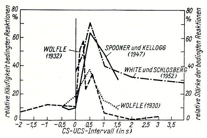
Fig.3-1: The influence of the time interval on the rate of formation of conditioned responses. CS represents a conditioned stimulus (e.g., bell), UCS the unconditioned stimulus (e.g., presentation of food; zero line). An optimum time for the development of a response can be observed in the range Δt = tCS - tUCS = 0.3...0.7 s. (According to Klix, Fig.6.5, p.368)
In Fig.3-1, we can imagine UCS as the ringing of a bell and CS as the presentation of food. In this case, a learning process can occur that develops excitation. If, however, part of the experimental box is put under voltage during CS, an inhibitory learning process will occur; the animal will flee this area after the bell rings.
In all cases, the learning success decreases with increasing Δt. For values of Δt < 0, learning success is almost nonexistent.
It becomes clear that learning can never be a single, isolated process. It always involves at least two distinct inputs, with the announcing input (bell) preceding the reward (food).
When we discuss learning in relation to interference networks, we will limit ourselves to the most basic principles for the sake of clarity. Weight learning and delay learning should suffice as such.
Donald Hebb, a student of Karl Lashley and a colleague of Karl Pribram, formulated a first fundamental learning hypothesis ("Hebb's Rule") that still dominates the ANN-world today:
"When an axon of cell A is near enough to excite cell B and repeatedly or persistently takes part in firing it, some growth process or metabolic change takes place in one or both cells such that A's efficiency, as one of the cells firing B, is increased."
Hebb, D.O.: The Organization of Behaviour. J. Willey & Sons, New York 1949
Hebb's Rule names weight learning. Is weight learning also applicable for interference networks in which delayed pulses interact - that is, for nerve networks?
Hebb's Rule says nothing about dynamic addressing or a delay structure. While neural network research (NN, ANN) has been deriving mapping principles via modification of weights (everyone, from perceptrons to SOM) for forty years, delaying pulse networks can only generate their mapping on the delay structure of the network. But we found:
Weights cannot withstand addressing due to delays!
For the example in Fig.2-1, there is no weight constellation that can reverse the assignment of the code pattern (case 1 or case 2) to the neurons! Delays are stronger than weights. Primarily there are delay addresses in a nerve network, only these can be used for weights learning.
Weight learning in delaying networks can only be done on an existing delay structure. If the delay structure does not exist, nothing can be learned.
This means: If codes are sent to a network that do not have any delay addresses in the network, the codes fizzle out. Nothing happens.
This realization produces a general rethinking of Hebb's rule:
If we assume that the delay time of a neurite grows towards a target, the delay structure is no longer correct when the neurite arrives at the target; the target address is then possibly wrong. This means that a network with (delay) addresses must first exist before learning can take place where an address already exists!
Ultimately, it means that a first process must be that of the growth of a (of whatever kind) nerve felt, and a second process that of (weighted) learning, and only in those places that already have an address. Synapses then only arise there.
If there is no address location for a time pattern, this pattern cannot be learned, ie the IN does not react to this pattern. (The address is understood to be the temporal pattern that can excite an address location.)
Conversely, this could result in:
If there is no time pattern for an address, the address can not be learned.
That would be a plausible, modified Hebb's rule adapted to pulse interference. The view corresponds to findings of individual genesis. Karl Pribram sent me a picture of Pomerat's findings. There, Pomerat 1964
(Fig.2-2, p.29 in Pribram, Karl: Languages of the Brain, 1971) described a felt-like sprouting of the nerve endings (growth cones). Download Karl Pribrams book as
PDF (17 MB).

Fig.3-2: Fig.2-2 of Pomerat. He differentiates between stochastic, felt-like growth and synaptic generation/degeneration.
Pribram differentiates between stochastic, felt-like growth and synaptic generation/degeneration. Synapses are only strengthened where they are needed. If sprouts or synapses are not needed, they degenerate again.
By the way, Pribram mentions an extremely explosive detail on page 31:
"Since fiber diameter is often an indicator of the length of the fiber, the thickening indirectly suggests that growth may have taken place." p.31
In other words: As a nerve fibre gets longer, it also becomes thicker. But growth in thickness means: it becomes faster. This can only mean one thing: This fiber is trying to maintain its signal delay!
If we remember the growth of our children, the growth process had its setbacks. Abrupt behavioral changes occurred. Were these the points at which the delay architecture of growing nerve fibers could no longer keep up and became confused?
Here we also receive a criterion for assessing the performance of neural learning algorithms. If code patterns of an algorithm match delay addresses, it is potentially able to simulate nerve networks.
All other algorithms don't have much to do with neural networks; they belong to the realm of "Artificial Neural Networks" (ANN).
The self-organizing map of interference networks is the addressing via network-immanent delays.
However, since the delay structure of the network is spatially fixed, this means a three-dimensional bond and a certain physicality. "Form codes behavior" wrote the author in the preface to 'Neuronal Interferences' in 1993:
If the network wants to learn, it must be checked before the learning of weights whether the required delay addresses are available.
There is a sad story about this finding. In 1990, thousands of completely neglected toddlers from Ceaucescu victims were found in Romanian children's homes, who had hardly any contact with anybody. Children who were more than two years old at that time will suffer from chronic behavioral deficits for life. Apparently, the basic structure of our nerve network develops in the first two years.
Because the address space (as a delay structure) results from a three-dimensional physicality of delaying interconnects, it will only adapt to changing patterns within a modest extent. Changes in the conduction speed are conceivable through slight variations in the diameter or length of a fiber. If the pattern or network changes beyond adjustment limits, what has been learned disappears forever, even if the learned weights are completely retained: knowledge, coordination or behavior can suddenly no longer be accessed.
This fact gives an indication of diseases in which the myelin sheaths of nerves degenerate and nerve fibers become drastically slower. In multiple sclerosis (MS), the delay structure of the network gets mixed up. Codes no longer reach the actually addressed neurons.
If, during the course of a spontaneous recovery from MS, everything suddenly starts working again, that would mean that the weights have outlasted the disease. But the author has no knowledge of whether such cases exist.
Karl Lashley, at that time the head of Donald Hebb and Karl Pribram at the Yerkes Laboratory for Primate Biology in Florida, studied learning with animal experiments. In his search for storage locations of a learned behavior, he was able to remove different areas of the cortex of rats without destroying learned information (path through a maze). After 30 years he came to the ironic conclusion that "what has been learned is not stored in the brain". He, of all people, was the first to speak about interference patterns. Karl Pribram writes in 'Brain and Mathematics' on page 4:
"Lashley (1942) had proposed that interference patterns among wave fronts in brain electrical activity could serve as the substrate of perception and memory as well. This suited my earlier intuitions, but Lashley and I had discussed this alternative repeatedly, without coming up with any idea
what wave fronts would look like in the brain. Nor could we figure out how, if they were there, how they could account for anything at the behavioral level. These discussions taking place between 1946 and 1948 became somewhat uncomfortable in regard to Don Hebb's book (1948) that he was writing at the time we were all together in the Yerkes Laboratory for Primate Biology in Florida. Lashley didn't like Hebb's formulation but could not express his reasons for this opinion: 'Hebb is correct in all his details, but he's just oh so wrong'."
Today we know that a neuron can only become active where all partial waves of a sending neuron arrive at the same time. In various essays I wrote
"Delays dominate over weights".
Weight learning without delays as the basis of an artificial neural network theory (ANN) inevitably leads to a completely different behavior compared to the nerve network.
Lashley apparently already sensed the interferential blockade of weight learning through delay addresses. He may also have suspected, that wave interference can only lead to one type of interferential learning. Be that as it is:
Hebb's Rule is limited to weight learning and is therefore only valid on a network with pre-existing delay addresses, or on a delay-free network. But this does not exist in nature, it only exists in the computer as ANN.
Or in the words of Karl Lashley: 'Hebb is correct in all his details, but he's just oh so wrong'.
Hebb's Rule led directly to Artificial Neural Networks (ANN), whose behavior has anything to do with that of nerve networks. For more details, see the page about the holographic brain.
One problem with applying Hebb's rule is that ANNs work with long-range effects that do not exist in the nervous system. The algorithm controls weights in an infinitely short time, delays play no role and were replaced very early by (computer) clocks by McCulloch/Pitts in 1943. See details in
"McCulloch/Pitts initiated a misdevelopment"
(german), (english).
The crucial question is where local information can come from, which a neuron needs in order to be able to change a delay or weight of a certain path.
Where could local reward incentives come from?
Infinitely fast long-range effects are not known in the nervous system. Nerve conduction speeds are very slow compared to electrical signals. Unlike computers, they cannot be controlled remotely.
Just as important is the question, unanswered by Hebb, of how inhibition can arise in the form of inhibitory synapses. They too have to be initiated locally.
In Chapter 14 we will turn to the recognition of tones and harmonies. Dr. Friedrich Blutner had a substantial suggestion for this: the hearing of professional musicians can perceive absolute frequency deviations of a few Hertz, this is referred to as "absolute hearing".
Since frequencies or sequences can in principle only be realized with neural delay times, the question arises as to how a nerve cell can adjust a delay so precisely that such recognition performance becomes possible.
Sequences in sporting competitions must be evaluated in a similar way. The diver, the gymnast or the football player have to carry out complex actions to the hundredth of a second. The more precisely the athlete masters the timing, the higher the chances of success.
The question now arises as to how a neuron or part of a neuron (the soma, an axon or a dendrite) can adjust or specifically change the delay of passing impulses. (All learnable, dynamic processes, i.e. speaking or hearing, sequences and movements or sound, speech and noise detection of all kinds, prove that this must be possible in principle.)
In addition to a change in structure through Hebb's Rule, a local control process is required that can adjust an individual delay within limits. If we think of the greatly varying thickness - and thus the variation in the conduction speed of different axons and their ability to conduct even faster through myelination, this question immediately arises.
If we think of neuron models in the style of Hodgkin/Huxley, countless parameters would come into consideration. In addition to ion concentrations, the length and thickness of dendrites and axons as well as the myelination of the axon are also important.
So how should a dendrid or an axon know that it should conduct more slowly or more quickly?
There is a possibility in the area of the structure of the network. It would be conceivable that a (multipolar) nerve cell, whose dendrites randomly connect to other cells that often act coherently with each other, controls the growth in thickness of the pulse-carrying dendrites in such a way that impulse extinction (due to the refractory phase of incoming impulses) can take place in the soma (analogous to impulse extinction in the sciatic nerve). It would then always fire when these nerve cells fire at different times but coherently with each other.
In this way, previously completely independent processes could be linked together. Also this is what creates dynamic plasticity, the nerve cell adapts small delay changes.

Fig. 3-3: Mask M and complementary mask M' of a simplest interference circuit consisting of two neurons (mask M refers to P, mask M' to P'). A pulse from neuron P is supposed to trigger excitation of neuron P'. If both neurons have identical topology, pulse transmission would be impossible. Source Chapter 4 from the "Biomodels" page
If we assume that the locations A and A' to D and D' are identical, it is noticeable that the corresponding delay times must be very different. Thus, length and delay PA is not equal to P'A' and so on. If any communication has to occure, the fibres have to be of very different thicknesses. The principle of neighborhood inhibition (Link) becomes clear. Neurons that are close together, generally cannot "talk" to one another.
Here we only consider the right-hand side of Fig.3-2. In order for neuron P' to fire when P emits pulses, the mask M' of P' has to be exactly equal to the complementary (time-inverted) mask M of P.
From this, a rule can be derived that can only be implemented locally and does not require any ominous long-range effects in the style of ANN. The resulting local rule for adjusting neuron P' for optimal delays would be:
A pulse that arrives later than the others would cause the relevant dendrite to grow in thickness or decrease in length. On the other hand, a pulse arriving prematurely on the dendrite would cause an increase in the delay due to a decrease in thickness or an increase of length.
It should be noted that this rule assumes an overdetermination of the wave field, see Chapter 15.

Fig.3-4: Fine adjustment of delays. Incoming pulses a) and b) at a synapse arrive too early or too late in relation to the excitation of the neuron. The delay of the corresponding dendrite must be reduced accordingly for case b) or increased for case a)
The delay τ is equal to the distance s divided by the conduction speed v of the fiber.
τ = s / v
The conduction speed of the dendrite increases with its thickness d. The delay τ of the dendrite in question will therefore decrease with the fiber diameter d, assuming a constant length s.
τ ∼ s / d
It would be assumed that there is a biochemical process that causes the thickness of the dendrite to increase or decrease when an impulse arrives too early or too late.
But we know, that a nerve cell is fired by billions of impulses every day. Therefore a single group of pulses should not have any effect. Only constant repetition over days, weeks or months can bring about a gradual change in behaviour.
A competitive athlete knows what that means: only constant repetition of the same training unit will help to complete this dynamic fine-tuning and bring the exercise to perfection.
But that would only be the beginning. We need further knowledge about which local mechanisms can lead to excitation, inhibition or delay adjustment.
And a crucial question remains: How is it possible that such local changes lead to meaningful behavior? For the sound perception according to
Chapter 14.2, corresponding connections would be conceivable.
Andrew Packard discovered in 1995 that an interferential spread of excitation between chromatophores (coloring cells) of squid can be observed. This suffices for a very simple interference model. He observed color waves of spontaneous excitation [AP1995], see Fig.4-1. The special thing about it: The substrate has an almost homogeneous, constant speed of propagation, the waves resemble water waves.
 Fig.4-1: Waves of spontaneous excitation on an octopus with the spinal cord cutted.
Source:
Colour Waves on Squids - Andrew Packard's Squid Experiments - A Neural Net that can be seen with the Naked Eye
What we think we see on the octopus are waves. But what we really see are opening and closing chromatophores. So what is our wave abstraction? From physics lessons we know the one-dimensional, elementary description of a time function, e.g. in the form
f(x-vt) (see the site of animations).
Let us imagine many such time functions that flow in the mesh of a 3-dimensional network. Its nodes may make any links between incoming time functions (addition, multiplication...) and forward them. The refractory period prevents the wave from being sent back; it can only propagate forward.
Andrew was also able to film waves that converge on one another. They also die out at the point of impact due to their refractory period.
Let us assume that our network is at rest and we excite a single node with a pulse. When we zoom out of this network, we can observe pulse propagation in the form of a ball-like wave that spreads around our node. However, it would only be observable at a homogeneous conduction speed, e.g. in acoustics or with Andrews Squids. In the case of inhomogeneous conduction speeds and an inhomogeneously designed network (cortex), the idea becomes more difficult. The visual impression of a spherical wave will quickly give way to that of a spherical chaos. Be that as it may: We notice that the one-dimensional moving time function in the n-dimensional area resembles a wave - even if we can no longer see this with the naked eye in the case of inhomogeneity. Hence the name: waves on wires.
We call a 'time function wave' an elementary abstraction of the temporal shift of information (here: pulse) in a network or in a medium.
Networks whose function is largely defined by the delay in the transmission of information are referred to as interference networks.
Why do we care? Because in 1993 it was discovered that these interference networks have imaging properties. Andrew's squid experiments are suddenly in a row with known, mirror-inverted images in the nervous system (homunculus; visual cortex etc.) via the aid of interference network theory. One conditionally affects the other:
Wherever an image can be found, wave propagation is the cause; imaging projections are to be expected, where wave propagation is to be found.
Incidentally, this sentence also applies to optical or acoustic images.
Let us consider that a single interrupted, electrical conductor path in the car leads to equipment (blinkers, headlights, horn, radio ...) no longer working, and let us also consider that a nerve cell is only about seven years old, we on the other hand, seventy-five on average, then a problem becomes apparent. At seventy-five, not a single nerve connection would work in our body. We would neither feel the hot stove, nor could we take our hand away.
As a result, we cannot afford a simple 'bell wire' connection between sensor/actuator and brain. Every nerve cell needs many double (s). Maybe we lay each line several times? Or do we solder all the lines together at all the plugs? From now on, headlights, starters, indicators, window lifters and horn would be activated when we press the wiper switch.
Or does the defective line repair itself?
In principle that would be possible. If it weren't for the learning of the necessary cross and cross connections: muscles should be tensed when standing up, others should be tensed when sitting down, and still others should be relaxed when standing up and sitting down. The biological network is interconnected a million times.
So if we have to do the task without individual bell wires - how do we get even a single piece of information in a chaotically interconnected, short-circuited network of neurons: "Please bend down!" At the same address (right index finger) for seventy-five years?
A neuron does not have an internet-IP address. In nature there is no protocol available with which information can be sent specifically to a target. It is also generally unclear to the sender which goal the data should achieve if neural learning is to be possible at various points in the network.
So how could a solution be?
In a cross-connected network (short-circuited everywhere), apparently only signal propagation times can connect the source and destination of information - via interference integrals. To do this, we have to send out every piece of information (pulse wave) in all directions. Where several pulses from a sender happen to arrive again at the same time (colloquial: interfere), a higher effective value arises - the goal has been reached
[NI93].
This can also be several goals at the same time. Or goals staggered one after the other. In contrast to the WWW, the origin and destination address of information in nerve networks can only be defined via the geometry of the (inhomogeneous) delay space. All delay-changing units can be regarded as 'switches': glia potential, chem. messenger substances, synaptic strength (this changes the time constants), inhibited or excited nerve cells as detours, stretching and compressing fibers (see thumb experiment).
As a result, a new computer science arises: In contrast to the Internet PC, the nerve cell does not know to whom and where it is sending its data. Even we cannot observe it, since all information initially disappears in all directions - but only interferes positively with itself again in a few places.
Do we have the slightest idea what it means to understand such computer science? Only when this interferential computer science has been sufficiently validated should we begin to interpret consciousness or intuition. Everything else is charlatanism.
When the idea was born in 1993, see annual reports or the project directory, it was initially uncertain whether the points of view were correct. The simulation of a wave field in the head is generally beyond our imagination. Simple detection experiments had to be developed. So the idea arose to write the simplest simulator that can simulate some essential properties of interference networks (Bio-Interface, later called PSI-Tools, at the end of this page).
We mentally took a bitmap with black pixels, acted as if the bitmap were a square pond without a border and the pixels were stones thrown into the pond and lowered three sensors (green) into it, which record the wave movement of the pond surface as a function of time. This then results in three time functions, see second picture. The first question was: Do these time functions actually contain the image of the bitmap? Can the generator image be read out again from the recorded time functions ? And under what restrictions is this possible?
5.1 Generator Field

Fig.5-1: Bitmap as generator field: Black pixels fire.
Let stones be thrown into a pool one after the other at the locations of the black pixels. Waves propagate in a circle around the emission locations and finally reach the sensors shown in green at the borders. The time functions of the wave field may be recorded at the three sensor locations marked in green.
5.2 Time Functions (3 channels)

Fig.5-2: Resulting time functions of the bitmap for the three sensor locations (the time axis points to the right).
We can see different time functions (blue, green and red) that have spikes at different points in time. The pulse image should be transmitted in three channels (we think of axons).
5.3 Reconstructive Interference Integral
The time functions are then passed into a second (wave) pond at defined locations (black). (In the case of interference reconstruction, in principle backwards in time). However, its x, y coordinates of the feed locations were chosen to be slightly different from those of the sensor field. The transit time on the three interconnects is assumed to be identical here (equal length, zero). The pulses now interfere with themselves at the original source locations (we call this self-interference) but also with predecessors and successors (called cross-interference or aliasing). The self-interference generates an interference integral in the form of the "GH". Cross interferences create the additional emissions that are visible around the self-interference image.
The computer allows us to choose the time direction for calculating the interference integral. If we want to test into the channels from behind, so to speak, we choose a backwards running time or negative delays and get what is known as an
interference-reconstruction.
If we are interested in a mapping that actually takes place in a nerve network, we select forward time and get what is known as an
interference projection.
With otherwise the same parameters, the reconstruction and projection are exactly mirror-inverted to one another, ie the reconstruction appears the right way round to the original, while the projection is mirror-inverted (see also a note below). Nature only knows the (mirror-inverted) projection, the (non-mirrored) reconstruction necessarily requires the computer.
 1994")
Fig.5-3: Three-channel interference integral from the channel data Fig.5-2 from November 14, 1994 - historically one of the first successful interference reconstructions (PSI tools). The source location at the bottom right has been moved so that the original image is reproduced in a distorted manner.
The coordinates of the right channel in Fig.5-3 were shifted up/in from the lower right corner to see how the interference integral reacts. There was simply a lack of imagination to imagine how a simple integral would react to distortion of the source geometry.
At that time there was a huge challenge in computing time: this image calculation took about a weekend, the first movies took a week. If the wrong parameters for exposure or reconstruction were chosen, everything started all over again.
A receiving space that is spatially different from the sending space can be used to check the superposition of pulses (interference) in target spaces of deviating geometry. An integration via the excitation of each location (interference integral) records the interferences that occurred at different times in the image. The simulation shows the conditions under which a receiver can reconstruct the transmission locations (transmission addresses), e.g. sensory excitations, from channel data transmitted multiple times in parallel. In the image, the lower right electrode was pushed 10% into the receiving field, which is equal to the generator field, before the reconstruction was started; the interference image appears distorted to the top left.
As you can guess, these questions are based on those who are asked about GPS (Global Positioning System), Phased Arrays from SONAR or RADAR, or the questions that colleagues from SKA (Square Kilometer Array) or sonography devices answer were. Here, too, it is a matter of comparably simple interference systems of a technical nature.
After irritations with the theory of the so-called Neural Nets (NN), I delimited the research on (pulse wave) networks around 1997 as "interference networks (IN)". The cause was permanent misunderstandings during lectures or publications. Neither the approach nor the statements about the IN theory could be understood, as no corresponding knowledge was available. To date, interference networks are nowhere taught. My attempts to set up appropriate lectures at institutes of the Humboldt University in Berlin unfortunately came to nothing. Neither the motivation nor the content of the theory was understood.
However, since it was registered in the neuro-community that common approaches (with state machines and delay-free interconnects etc.) are obviously completely unsuitable for the description of nerve networks, the following more and more went over to the classic research field "neural networks" (NN) to be referred to as "Artifical Neural Nets" (ANN).
We owe the curiosity to this development that we have to designate the networks that deal with the modeling of nervous properties as interference networks, while "artificial neural networks" (ANN) with no run-time - especially in the years up to 1997 - were designated as "neural networks".
Even today, this confusion is fatal for student education. Open any book on neural networks: The introduction covers the biology of nerve cells, followed by the theories of artificial neural networks - which usually have no behavioral similarities of neural networks.
Survival in the animal kingdom is directly linked to the concept of recognition, think of ways to food or watering places, the visual distinction between poisonous plants and food, between cliffs and steps, between friend and foe, between large and small. Recognizable optical features, however, are subject to changes in distance and consequent constant changes in size and shape.
If you try to train a somehow weighted network with a face at a distance of one meter from the recording camera, this network will, under favorable circumstances, recognize the face at the same distance. Recognition will be impossible as soon as we change the distance to the face, rotate it, move it or tilt it.
How can we convince a network of nerves to recognize a face that appears at varying intervals? How could nature help itself?
We remember that the geometric wavelength
L = vT = v/f
(v: conduction velocity of nerve, T: pause duration between pulses, f = 1/T)
depends on the conduction velocity. If the conduction speed varies, the interference locations vary. But what does that mean in a mapping network? How can you imagine this variation?
We want to make an experiment similar to the one above. G-shaped pulse sources (eg neurons) serve as the generator. Again, the waves may spread out in a circle around the source and reach the three channels at different times. Again we project via the channels into the receiving field. Once in the target field, the waves spread out again in circles. Where they meet, our screen changes from yellow to red to blue. We only vary the speed of propagation of the waves in the receiving field (background velocity v).
As a result, we see that, depending on the selected propagation speed of the waves in the receiving space, interference integrals ("images") of different dimensions arise. Comparable to a photo lens, this effect is called "zoom".
")
Fig.6-1: Simulation of an interferential projection between two neural fields that are connected via three axons. The conduction velocity v of the detector field varies.
First publications in:
(Virex96) Fig.8 and
(Bionet96) Fig.9.
The figure shows a 'zoom'-effect comparable to optical zoom. As more we zoom out, as more cross-interferences came into the field. In Figure 5g) we see holographic properties and non-locality of neuronal memory (known from Lashley's rat experiments).
The time functions are generated in a generator space with a normalized speed v = 50 (in mm/s). The projection is calculated in a second, receiving space. The image size varies under the influence of the (normalized) master speed (v = 100, 75, 50, 20, 10) in the receiving space. a) Simulated generator field, black pixels pulse; b) resulting channel data; c) to e) Interference integrals over the channel data, the parameter is the background speed v. If a speed that is identical to the transmitter a) is used, a mirror-inverted image is created on the same scale d). If, on the other hand, the background speed is changed, the image 'zooms', see c) and e). Interference arises in the receiving field where the pulse waves of all three channels arrive at the same time. If the coordinates are assumed in cm, for example, the speed results in cm per second (pulse width 2 ms, sampling rate 5 kHz).
Now you may be wondering why we have put all this effort into? To this end, we remember the (neuro-) glia as a supply substrate for the nerve cells. It is known that the glia influences the conduction velocity of nerve fibers passing through it. We can perceive this via electrostatic conductors: When the conduction speed changes, the measurable potential of the glia changes at the same time. If we measure potentials at the cortex with the EEG (ECoG), we can assume that different potential regions have different conduction speeds - no more and no less (see also the
EEG-experiments page).
Since it was already pointed out in the book "Neuronal Interferences" (1993) that a variation of the conduction speed in the transmitting or receiving field influences the scale of the mapping between the two, it was obvious to develop a scenario for this simulation.
What we see here is nothing more and nothing less than the effect of a potential field in the EEG: the images below begin to zoom. And the gradient at the edge could even cause an offset (see
movement).
EEGs therefore have nothing to do with nervous data. We see focusing voltages for projections between neural fields, the technical utilization of which could lead to the defocusing (derailment) of the overall system. (Incidentally, this realization stopped own ideas for technical applications of EEG in 1997.)
But it should also be remembered that certain squids do not have the chance to zoom. They only recognize prey if they appear at the right distance in front of them. The background seems to be more of practical nature.
(Note: There is a further supplement to this section in
deutsch and
english)
Lashley was looking for the location of memory contents. He trained rats to find food in a maze. Then he systematically removed grid-like small parts of their brain and observed the effect. Whichever part of the cortex he removed, the rats remembered what they had learned more or less well.
After 30 years he resignedly confessed that he was no longer sure whether the brain was really the place of the memory: "The series of experiments ... has discovered nothing directly of the real nature of the engram", he noted (K.S. Lashley: "In search of the engram". Cambridge Univ. Press 1950, Ch.5, p.62).
And yet, making this experiments Lashley had discovered something extremly crucial: Apparently memories can only be holographically encoded in the cortex! So let's take a look at the following picture:
Fig.7-1: Simulation of a three channel projection in a two dimensional space.
Coming from the three "axons" K1...K3, the time functions (pulse waves) flow across the field. Wherever pulses meet, the interference integral value is higher, we see small red peaks as potentially locations of storage.
To simplify things, it is assumed here that the pulse waves should move at a constant speed - the simulation shows only the general principle behind delays of wiring producing cortical hologramms.
We find holographic properties and the non-locality of neuronal memory (known from Lashley's rat experiments). Around the central, self-interferential "G" we find all the cross-interference figures. They contain parts of the central "G". The pixels of the "G" have been relatively dense several times sent over and over again.
David Bohm and Karl Pribram discussed holographic organizational possibilities since the 1950s. Karls student Walter Freeman even gave a fictional image of a wave field in his 1972 work: Waves, Pulses, and the Theory of Neural Masses (Progress in theor. Biology, Vol. 2, 1972, New York/London).
As luck would have it, self-holographic maps were immediately visible during the first experiments with zooming images, see
Fig.6-1, g) or the GFaI-Annual Report 1994, Bild 4,
(PDF).
Holomorphy (or holography) is inherent in the nature of interference networks.
In Fig.6-1, g) we see, that not only the picture of the original, a capital "G", is mirror-inverted in the detector space, but many, incomplete G's are also mapped around it. The realization: A neural map cannot be saved in just one place. It is always stored holographically!
However, only low-channel projections map directly holographically
(d = k+1). A too high channel number k in relation to space dimension d eliminates the cross-interference (this is why acoustic cameras require high channel numbers). But every high channel-number projection addresses low channel number projections too, so in general, all neural projections are holographic.
There was a prediction for this in the book 'Neuronal Interferences' 1993, but without simulative evidence it was worthless. Since the holographic term for sinusoidal time functions of an optical type was occupied in a specific way with reference waves, the property shown here was referred to in [NI93], Ch. 5 als tutographic mapping** - tuto : safe, protected.
Holography or tutography?
When Dénes Gábor invented holography in the forties, it was created in the color space of light, in the Fourier space. However, if we apply the Fourier transform to pulse-shaped time functions, nothing clever will come of it. It should be noted that the concept of interferential tutography is open to any kind of time function (Dirac to sine, code pattern or sequence of states), while holography is always associated with sinoidal time functions, think of the well-known light spectrum.
This means that (interferential) tutography should be viewed as a generic term for holography, which is also existent in the time domain.
Let us look again at the zoom image Fig.6-1, g). While only a mirror-inverted 'G' can be seen in images (c) to (e), further interferences enter the image field in images (f) and (g). Apparently the following pulse waves now interfere with each other and with the original pulse wave. The result is fascinating. We find the same interference integrals of the 'G' all around! Image (g) consequently shows a kind of hologram as a fundamental peculiarity of interferential images.
Suddenly Lashley's rat experiments can be interpreted: interference networks store holographically (better: tutographically) and Lashley provided the decisive evidence for this! Lashley's unsuccessful search thus becomes important evidence of an universal, interferential effect in the nervous system!
Neuroscientists Lashley, Pribram, and Hebb had noticed Gábor's idea of holography. When Karl Pribram met Dénes Gábor years later at a UNESCO conference, he explained his holographic brain analogy to him. He wrote about this in "Brain and Mathematics" 1971:
Gabor was pleased in general but stated that "brain processing [of the kind we were discussing] was Fourier-like but not exactly Fourier." I asked, what then might such a relation look like and Gabor had no answer.
The interesting thing about it is the phrase "but not exactly Fourier". Gabor suspects or knows clearly that a Fourier transform of stochastic pulse patterns can bring no meaningful results. At that time all holography takes place in the optical spectral space. Holography in the time domain does not even begin to exist, Fig.6-1, g) was not possible to make before the 1990's). What Gabor wanted to express was something like: Fourier and holography go well with optics, but not with the nervous system. To understand Fourier better, remember that the spectrum of light - its Fourier transform - can be generated with a simple prism.
If we take a closer look at the result of the simulation, we can see that pulse projections not only map a "G" onto a "G". Rather, many more "G" appear around a central "G". The originally unique information "G" in the generator field is mapped several times in the detector field - but why?
To understand it, let us recall the two possible types of interference:
1) On the one hand, identical waves of the pixel p can interfere with one another (waves i, i, i). This emphasizes the location of what we call self-interferences, the location of the desired "image" of all pixels - our mirrored "G" in the center of the image.
2) In addition, however, all waves (i, i+1, i-1, i+2, i-2 ... ) of all channels interfere with each other somewhere in the running period. We will call meetings of waves with different indizes cross-interferences. If, for example, the i-th wave of channel 1 meets the (i+1)-th wave of channel 2 and the (i-1)-th wave of channel 3, one of the figures of the innermost circle is created. The resulting interference patterns appear similar to the original. Other combinations cause the further cross-interference figures. The "G" is consequently inevitably projected not just once, but multiple times into the detector space. We recognize the (average) pulse interval in the time functions
[NI93]
and the wavelength of the pulse pause or the cross interference radius R based on this as a measure of the distance between self- interference and cross interference locations.
How is the actual distance R between the recurring 'G'
in Fig.7-1 defined? For this we remember that there are only places in the interference integral that have a high effective value. These are exactly the places where waves meet.

Fig.8-1: If a pulse-wave hits its own twin brother (colloquially itself) at a defined location, we speak of self-interference (a). If, on the other hand, it encounters a predecessor or successor pulse, we speak of cross-interference (b). Source: [NI93], Kap.2a, S.52
Self-interference is essentially about cross-correlation of a time function with itself. Cross-interference could remotely be thought of as autocorrelation.
This is exactly where "hearing" and "seeing" differ fundamentally: Projections (pictures, imaginations) are self-interference images (a), while temporal structures (pitch, sounds, language, etc.) can only be generated with cross-interferences (b).
But if we look at relationships within images (textures, patterns, affiliations), then we are at cross-interference in the picture: We recognize an object through cross interference! So seeing is also hearing.
However, so that one place can get a higher effective value than any neighboring one, care must be taken that as many waves as possible from different directions meet exactly at the place.
But every wave has a predecessor and a successor. So if many waves meet in one place, then their predecessors and successors are also in well-defined places - shortly before or shortly after.

Fig.8-2: Meeting locations of waves correspond in the interference integral with excitation locations. Consequently, the cross-interference radius can be determined from the wave field. It results from the distance between successive waves with wavelength λ = 2R. (Sorry: a 4-channel wave field is drawn on the left, while a 3-channel interference integral is drawn on the right).
So we found a relationship between the average pulse pause T of the time functions at (maximum) rate of fire f and the center-to-center distance of the interference locations (cross interference radius) R.
Let the wavelength λ = vT with v: conduction velocity and T : pulse pause, waves in opposite directions interfere with each other again at half the geometric wavelength. Consequently, there is a relationship between the average wavelength λ and the cross-interference radius R [NI93]:
(1) R = λ/2 = vT/2
With a fire rate f = 1/T we find
(2) R = v/2f
or, if we want to determine the expected conduction velocity from a fiber density
(3) v = 2f R = 2f λ/2 = f λ.
In an interference network, the parameters of the conduction velocity v, the cross-interference radius R, the rate of fire f, or the pulse pause T = 1/f are obviously inextricably linked. If a system has a cross interference radius specified, for example by somatotopia, then a well-defined velocity belongs to it. If a velocity can be measured, the size of the somatotopic area can be estimated from it.
However, it should be noted that the partial pulses generally arrive at fibers of different thicknesses. The guiding speed varies greatly in proportion to the thickness. In this respect, the above formulas are only approximations for an averaged velocity.
Calculation example: The Swiss Guardian
If we want to trigger a movement in the little toe, then any cross-interference on the path from the cortex to the toe must be excluded so that other areas of the body are not also stimulated.
How high should the guiding speed v be, so that the places to be addressed in our body are not overlaid by cross interference? We assume that the nerve network under consideration has a maximum fire frequency fof approximately 30 Hz, and that the individual is nearly two meters tall (Swiss Guardian) - with this we need a cross-interference distance
R of approximately 2 meters. This applies to both ascending and descending impulses.
R = 2m
with R = λ/2 follows
λ = 2R = 4m,
so we require a velocity v of
v = f · 2R = 30Hz · 4m = 120 m/s.
If we look at known
fiber conduction velocities this would correspond to a type "Aa" according to Erlanger/Gasser or type "I" according to Lloyd/Hunt. It is the fastest type of fiber, it is myelinated.
Should we note, that examples on this homepage match known values from the nervous system: Can this be a coincidence? Probably not?
Discussion
-
If the pulse pause increases, the cross-interference distance increases and larger areas can be more clearly addressed.
-
If the rate of fire increases, the cross-interference distance becomes smaller (see pain simulation) and the images become blurred.
-
If the velocity increases, the cross-interference distance increases and larger areas can be addressed.
-
If the routing speed is lower, the addressable grid becomes finer, more information can be accommodated per volume unit (see
storage density).
It is important to note here that cross-interference as well as self-interference have independent tasks to perform and that they complement or exclude each other depending on the task. For more information, see
[NI93] and later papers in the
list of publications.
In the case of interference integrals, the image content is always in relation to the parameters of the time functions, conveyed via the cross-interference distance or radius (see above): Around a channel (ganglion) it is only possible to project aliasing-free into an area whose radius is not larger than the average cross-interference distance (geometric length of the pulse pause).
The following examples do not claim to be correct, they are to be understood as a hypothesis in which direction the matter to be analyzed can be researched. Further analyses of code selection using delay lines were already described in a very concise form 1993 in
Chapter 8b of the book "Neuronal Interferences" (German).
Example 1: Model of retina
Let us assume that the average pulse pause between successive pulses is T = 20 ms at the maximum fire rate. The pulse width should be negligible and the average, radial guiding speed is v = 1 mm/s (including synaptic processes; arbitrary assumptions). We calculate an cross-interference radius of R = vT/2 = 1 mm/s · 20 ms = 10 µm. This means that the distance between two ganglia in the source or sink area can not be greater than R = 10 µm, in order not to lose information due to cross-interference overflow.
If the ganglion root distance in the area of the retina (~ 100mm²) is about 1,000,000 / 100 mm² = 10,000 / mm² = 100 · 100 per mm², the result is an cross-interference radius per ganglion of slightly more than R = 10 µm, see calculation above. We find the neural grid exactly in this order of magnitude. Can it be a coincidence again?
Example 2: Model of the visual cortex
In the visual cortex (VC) a much larger area, almost 100 cm² = 10,000 mm², has to be covered with the fiber bundle of the optic nerve. As a result, a different background velocity is required here in order to prevent interference overflow. The fiber density is F = 1,000,000 / 10,000 mm² = 100 per mm², the cross-interference radius (= fiber spacing) is here approximately R = sqrt(F) = 100 µm. According to eq. (1) there would be a guiding speed in the VC of v = 2R / T = 2 · 0.1 mm / 20 ms = 0.01 m/s = 10 cm per sec. It should be possible to measure this difference experimentally.
 Example 3: Units coupled in the cortex
How can a connection to another part of the cortex be established with this cross-interference distance without us violating the cross-interference condition? (Only 100 µm are allowed?)
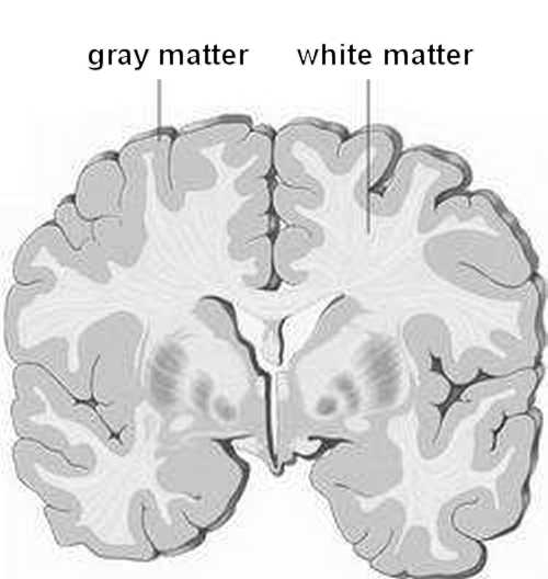
If we want to achieve an cross-interference radius of 10 cm, we need a background speed of v = 2R / T = 2R f = 2 · 100mm · 50Hz = 10,000 mm/s = 10 m per sec (f: maximum fire rate, arbitrary assumption here 50 Hz). But for this we need a myelination of the nerve tracts. This is visibly grayer than the non-myelinated areas, see the sectional view of the cortex. Just pure coincidence again?
Example 4: Body projection to the little toe
If it is to be ensured that a skin surface is mapped unambiguously in any cortical area - avoiding cross-interference, that can lead to confusion (the individual would not be able to clearly assign sensory excitations), it must be ensured that the cross-interference radius R is large enough in relation to the mapping surface is. So for an cross-interference distance R = 2 m (distance cortex - toe) with an arbitrarily assumed fire pause 1/f corresponding to f = 30 Hz, we would need a conduction speed of v = 2Rf = 2 · 2m · 30Hz = 120 m/s. Do we now think of the conduction velocity of peripheral, myelinated nerves? This is in fact around 120 m/s. Pure coincidence again! Of course, these are only rough guidelines. We know in detail that the most varied fiber speeds are encountered, the nervous system is seriously inhomogeneously interconnected.
But what does this coincidental coincidences mean? It can only mean that nature found a solution to the unsolvable question to avoid bell wires: In order to save interconnects, not only the cortex, but also the so-called peripheral nervous system is (partially) interferential interconnected.
Example 5: Multiple sclerosis
The clinical picture of multiple sclerosis can be analyzed from the point of view of the interference networks (cf. NI93). In this disease, among other things, the conduction velocity of myelinated (generally peripheral) nerves decreases. Since the geometric wavelength is equal to the conduction speed multiplied with the pulse pause, the geometrical wavelength is reduced. Cross-interference maps move into the area of ??the self-interference maps, see pain model. This means that peripheral actuators (muscles) and peripheral sensors (sense of touch, etc.) can no longer be clearly addressed/controlled/assigned, see example 4. Cross-interference creeps into areas that should actually be clearly addressed by self-interference.
From the theory of IN, the fatal consequences can be predicted, which again coincidentally coincide with the medical findings: from a sensory point of view, ambiguities in the interpretation of place assignments are to be expected. Motorical we can expect, that every wanted muscle adressing produces unwanted excitements of other muscles at unwanted places. Cramps and twitching would be the result (spasticity, tremor, pain). A simulation of the process is very close to the
pain model.
As a remedy, drugs could be used, that increase the conduction velocity v and/or that extend the pulse interval T (as so-called refractory time), see equation (1).
Example 6: Short-term memory
We remember, that different cross-interference radii are coupled to different conduction speeds. And different conduction speeds are bound to different cell types, synapses and layers.
Let us ask, how a short-term memory comes about (Plato: pantha rhei - everything flows), and what this could be - after all, we want to suspect two minutes after the colleague's arrival that he is still behind us, without again having to turn us around - so we have a problem.
On the one hand, it can be assumed, that the completely different pieces of information, which are generally to be linked here, lay not in closest distance to one another in the cortex. Larger distances, however, need higher conduction speeds; if we take v = 2Rf = 20 m/s, to retain the self- interference map.
But to be able, to let a pulse run through the cortex for two minutes, we need the opposite: we need very low conduction speeds, perhaps v = s / t = 20 cm / 100 s = 2 mm/s. That would be a factor of ten thousand less.
One solution to the problem would be, to first bring the information quickly to where it can be linked and second, to couple it there into another interference network that is 10,000 times slower. However, this would then only have an cross-interference distance of R = vT / 2 = 2mm/s · 20ms / 2 = 20 µm.
What does that mean? It means nothing more and nothing less than that the coarse network (with 10 m/s) in the fine network (2 mm/s) can no longer separate any place. The location disappears during this operation, what remains is the time, is only the time reference! Our short-term memory can then only be interpreted as a degenerate, too harshly coupled interference network, from which the location assignment disappears.
Example 7: Hearing maps
If we do not want to analyse location assignments, but rather frequency-sensitive 'audio maps' or code-dependent behavior as an I²-map (I²: interference integral), we need exactly the opposite as before: we need the cross-interference (outside the self-interference radius), see above. We assume that when a tone is recognized, the self-interference integral shrinks to neuron format, so that it no longer needs any image-content. So we are only interested in the cross-interference map. It would be as if we zoom-out much further out of an image (g) with v = 100, eg with v = 1000. Then the "G" melts together to a single point and we see only the cross-interference map of the noise, for example.
To check, whether the proportions also correspond to the nervous reality, we do the following calculation. If we take (arbitrarily) from the auditory cortex a conduction speed v = 10 mm/s and a frequency to be mapped
f = 1 kHz, we get a radius of cross-interference
R = v/(2f) = 10 mm/s /(2 · 1000 Hz)
R = 5 µm
In fact, this cross-interference ratio is really suitable for reducing the self-interference mapping to neuron size! With this constellation, only frequencies, sounds or noises are mapped. They produce an image - but only of the sound. (Have we already understood the potential of this simple calculation?)
Finally, if we ask ourselves why primates hear in the frequency range between 100 Hz and 10 kHz, a new aspect suddenly comes into play: the geometry of the nervous system must match the frequency range so that the cross-interference maps fit into it. This also implies that animals can hear in other frequency ranges, for example dolphins or bats.
In place of a conclusion
Would you have thought, that elementary properties of a nervous system would be so easy to calculate? With every sample calculation I was surprised by the perfect fit of the proportions.
Have we already thought about why we can't see a car speeding by in single frames like in a film? What is different about our nervous system in relation to the technical world around us? Why is our thinking not limited to the two dimensions of the film image? Why and how do we perceive the n-dimensional world that surrounds us?
Since we have already recognized, that the destination of information in interference networks is not caused by wiring, but by delays, we want to look at the influence of a single delay on the interference integral. We choose a test setup similar to that used for zooming. G-shaped, pulsating pixels serve as the generator. The channels are again projected into receiving fields with forward running time. We calculate images for delays of a single channel from dt = +4 to -12 ms.

Fig.10-1: Interferential projection between two neural fields that are connected via three axons. In a three-channel projection we vary the delay dt of one channel. Image modified from GFaI annual report 1994, p.69, Bild 6
(PDF). Published in
(Bionet96), Fig.8.
For the simulation, a variable delay dt is switched into interconnect of a channel. We see that the picture in the receiving field begins to shift when the delay time of that channel varies. The center of the image shifts to the side of the higher delay.
The importance of this simulation can hardly be assessed. It is sufficient to change the conduction speeds or delays (dt) so that images in the cortex begin to wander or to move. Incidentally, we can measure the changes indirectly with the EEG: Changes in potential (EEG) in the glia cause changes in conduction velocity in dendrites and axons. In the EEG, we probably only measure steering potentials for zooming and movement. We do not measure information content in the EEG, but control parameters that determine the pathes of information! From the IT perspective, we do not visualize data in the EEG, but addresses!
Why is a homunculus needed?
(Homunculus as the projective fields for motor- and sensory information within the cortex).
When we recapitulate, that target areas of information in interference nets are given not via interconnects but via delays, and we remember Penfield's Homunculus, in which many target areas have to be ranked next to one another, we begin to suspect the tremendous achievement that zooming and movement has to provide. Only if each partial map is projected exactly into its target area does the overall system work without confusion.
If we remember, that in the
thumb experiment it was found back in 1992, that wavefronts orient themselves according to the alignment of the thumb, we also have an inkling of what the sensory and motor homunculus are actually needed for, and why both lie in a precisely defined strip of the cortex. In principle we could assume that the homunculus would be superfluous. But for what is this strange interface of the motor- and sensory body projections needed?
Let us assume that a stretching or bending of the spine - as with the thumb - causes the ascending (cortical) projection fields to give way to the sides. Then all the ascending, sensory information in the cortex would arrive in wrong places! Conversely, all descending motor information would also arrive incorrectly. Instead of the little toe, the thigh would move. To prevent this, special interfaces are required that use control information from the wave field to correct its field alignment. The
Homunculus
in the cortex is apparently used for this purpose. An standardized image, so to speak, with zooming and movement, is passed to these from both the cortex and the spinal cord for further processing.
The information leakage from the spinal cord is directed via an ingeniously simple,
hyperbolic projection.
The above figure also shows that simple, digital circuits would be able to move images (2D/3D) in space by changing a single interconnect delay. For nerve networks, this circuit provides a basic possibility of following an object parametrically to a certain extent or adaptively adapting its change in shape. (In the computer, image movements - as on the canvas - are resolved by completely different processes that cannot be compared with nature.)
(Abstraction for columns of the visual cortex)
Interferential projection forms a type of geometric coding when many channels are arranged close together in the source area. Around 130 million receptors converge on one million ganglion cells on the retina (eye), ie one 'channel' (ganglion) supplies 130 receptors. A corresponding, roughly simplified interference model shows essential, interferential properties of such structures. See the following 16-channel projection of a "GH" (below) onto an opposite area (above).

Fig.11-1: 16-channel projection. Information reduction between two corresponding interference integrals (I²). It seems to be also a kind of hologramm. Only published here in the web.
If a template is observed at suitable points, interference integrals can be developed, that can only be synthesized by very few neurons, see more in
Chapter 17.
The background is the possibility that in any spatial dimension (inhomogeneity) every mapping is decomposable and reducible to a neuron, for derivation approaches see
[NI93].
We discover Rizzolatti's
Mirror neurons
as a possible biological equivalent.
While our original image ("GH" below) may consist of around 40 firing neurons, we only see three strongly activated areas (peaks) above. These represent the picture below. If we were to include additional, inhomogeneous fibers, a single point of interference could be found that represents the entire GH. In other words: an abstraction and information reduction take place here. The complex GH below converges in the fire of three neurons above. The maps below and above interfere with each other, one is the counterpart of the other, for more see [NI 1993]
'Permutation' Kap.5, p.100 ff.

Fig.11-2: Equivalence of a higher-dimensional image on the left with three lower-dimensional images on the right. According to this principle, a single neuron can reference any complex mapping or sequence of states (we find it in the homunculus, for example). But strongly the principle works only in one direction, from left to right or from high to low channel numbers. Because any high-channel projection always has low-channel (holistic) parts, the rats of Karl Lashleys could mutually remember. Source [NI93], Kap.5, p.100, interferential coding by permutation. Published in
[SAMS94], p.157, Fig.11
Regarding the principle of permutations following [NI93]: If all transit times between source and sink between subspaces P12, P23, P34 and P1234 are identical, recoding is possible. Here three interference locations P12, P23, P34 of lower spatial dimension are bound by a location P1234 of higher dimension. We recognize a new problem: While the interconnection works from left to right, things do not work quite as well from right to left (see over-determination).
We either need a synchronization (hardly conceivable here); we have to couple in separately with the same determination ( k = d + 1 ) or we have to delay/integrate in time. At the moment one can only guess at the various meanings of this image for the neurosciences.
Interpretation for cortical columns
If we choose a local neighborhood of all neurons in the receiving field, we could choose parameters so that every one neighborhood is mirrored upwards around an axon ascending here. The upper map would then look as if viewed through a pane of glass structured with bubbles: the lower detail is reflected in each bubble, but overall the map is reproduced without a mirror. A column organization becomes visible.
There is much evidence that this is the reading of the visual cortex.
Another reading arises with global coupling, as shown in the picture. Completely different image qualities emerge here, indicating mechanisms of abstraction.
On the one hand, the picture illustrates the inevitable formation of 'columns' around ganglia; on the other hand, the 1:130 ratio can be used to determine all parameters that contribute to the calculation of the retina - ganglion - visual cortex interference system.
Since we know that a single neuron cannot distinguish whether it is processing information from the eyes, ears, nose, speech organ or locomotor organs - it is always only pulses that it 'sees' - we can create adequate models for speaking/listening or observing/performing movement. In all cases, a more complex interference integral is mapped to a more abstract one by means of interferential permutation (for more see manuscript Neuronal Interferences NI93). It does not matter whether the origin of the maps comes from cross-interference (audio maps, spectral maps, behavior maps) or from self-interference (images). Only the space-time parameters between the source field, channels and sink field are essential for the calculation.
How is it possible that millions of sensors in our legs project mirror-inverted onto the sensory part of the homunculus without wiring errors, without one or the other circuit error leading us to believe that the left big toe is right and vice versa? Does nature have a code at its disposal to interweave images of thoughts or to combine ideas with one another?
To check this, we simply add the time functions of three channels in each of two generator fields. We append the channel data sets of a before generated 'g' and a 'h'.

Fig.12-1: Projection of two generator spaces (above) onto one detector space (below). Black marked places pulse. The time function data sets of the generator spaces were appended before the reconstruction.
In the detector space, the images overlap in a most remarkable way. It can no longer be traced from which source image the respective excitation in the detector space originates. Here, for the first time, two images merge into one. As CS Peirce (1837-1914) remarked in 1902:
"All thought is in signs".
What does semiotics mean in relation to our interference integrals? The word heard forms a sound map, see above. This is associated with a pictorial map, called an idea of ??the object. Both can then still associate with a font card via permutation - however, it gets more complicated here.
In principle, time function bundles can technically be attached to one another (to append) or added to one another (to add). (Nerve cells can only add, not append). The difference between the two methods lies in the fact that the pulse spacing becomes smaller when adding up, roughly halving, compared to appending, with the consequence that the cross-interferences come nearer.
The more time functions are added per channel (several sensory impressions at the same time), the denser the pulse trains and the closer the cross-interference distances come into the picture. We all know this phenomenon. In the event of an accident, our thoughts roll over and we can no longer think clearly because the cross-interferences occupie the field of vision complete and confuse us. Because of field overflow, under such circumstances the nerve system is completely blocked, it is really not possible to do or to memorize anything, see details in the
pain simulation.
Until 1996, I was concerned with the question of what actually happens when we arbitrarily move the source locations of the channels around in the detector field. Since we cannot imagine such interference integrals, we have to simulate them. To do this, we again use the channel data set of the conjugate mapping from Fig.12-1 and change the source locations in the detector space.
")
Fig.13-1:
Topological projections in different detector spaces. Variation of the channel arrangement causes partial zooming and moving effects, partial image delimitation, image distortion or multiple appearances. The topological cohesion of the projections cannot be resolved. The images 'g' and 'h' merge inseparable.
The resulting interference integral locations look as if they are held together by a rubber net. It can be seen that neighborhoods do not tear apart. The local neighborhood is always preserved, it cannot be separated.
From the "movement" we learned that, unlike the doorbell system in interference networks, any wire does not indicate the direction of the flow of information. It is delays and it is the simultaneity of the arrival of several impulses that define the destination.
In interference networks, excitations arise only at interferentially defined locations. Consequently, the transit time, the source and sink as well as the (temporal) channel geometry of the transmission lines reproduce the mapping of a generator map onto a detector map. Any number of branches can be switched into the transmission lines. In the case of interferential transmission, the address of the data depends only on the location of the interference, never on the geometry or the fanning out of the pathways (nerve ramifications).
Note the problem, that arises with a fiber bundle that transports images. Parametric fluctuations in the conduction speed can cause a movement of the maxima in the bundle, which means that the desired mapping can arise wide outside the fiber axis. However, if the image physically leaves the neural space or the interference field, it disappeares.
It is to be feared that this problem will be the cause of many nerve diseases. Long before a nerve dies, its parameters change: And for our images to slip, a tiny change in the conduction speed or in the pulse pause is sufficient.
But if images slip, they slip out of the network into nowhere or in the network into a neighboring (partial) map: we can refer to the first case by analogy as forgetting, the second as confusion.
So maybe there is still hope for Alzheimer's and Parkinson's? Are both diseases initially of the same cause? If large areas of nerve tracts are affected, it is to be expected that images will initially become blurred or distorted as a result of the change in the delay time structure.
By the way, what does "out of the network" mean? Please remember that every n-channel interference location is defined by an (at least) n-digit mask with n delays. If a channel breaks due to a synaptic failure, the information would no longer be available (forgotten). That is why many more channels have to be involved. But be careful: reliability in the interference network is bought at the price of overdetermination (number of channels n > dimension d + 1)! And overdetermination limits the possibilities for zooming and movement.
13.1 Rule of Over-Determination
Are You Scientist, Musician or Boxer? If redundancy is required for injury reasons, high-channel imaging will be advantageous. But these suppress delicate, weak emission sources. As a scientist, you've probably already noticed: the worst ideas come at night, when you wake up at half past two and can't go back to sleep. The darkness ensures relative silence in the cortex. Even weak associations come to life now, we have great ideas, but they usually turn out to be not quite so brilliant the following day.
Completely different for a boxer. What does this mean, for example, for a boxer whose nerve network is permanently damaged by hard blows?
He has to train strongly overdetermined projections. (We don't know how he does it). If we think about the fact that a high degree of overdetermination blocks cross-interference and costs flexibility in zooming and movement, the boxer is in a hopeless situation:
Either his nerve network becomes inflexible (overdetermined) due to the blows received: he becomes the "taker type". Or he deals out blows, receives little, and remains mentally flexible (intelligent). If we think of the biographies of great boxers (Cassius Clay alias Muhammad Ali), we suspect that there "could be something to it".
13.2 Neural Diseases
If any conduction speed of any single transmitting channel in the picture above changes, the projection would immediately shift out (see movement).
In order to be able to transmit images efficiently (think of the retina - the visual pathway - the visual cortex), one million fibers must have exactly matched transit times or conduction speeds. If not, a map moves into an adjacent map and there is confusion, see above. It is an interesting task for neurobiologists to investigate which mechanisms actually ensure this adjustment.
Multiple sclerosis is an example of what happens when the conduction velocities change. Synapses or nerve fibers may also die here. However, as a result of slow myelin dissolution (insulation of the fibers), the conduction speed changes measurably, it decreases, fibers that are no longer myelinated become slower by about a power of ten. If this process does not take place uniformly in a fiber bundle, interference locations wander or zoom out, or the images disappear. This is called paralysis.
Quite apart from the fact that the cross-interference radius then becomes smaller if the rate of fire remains the same - the system can then no longer clearly identify or control locations. Medicines that reduce the rate of fire would help. Incidentally, from the point of view of the interference networks, these are painkillers - see the
pain simulation for more.
Aha, you might say now: Apparently muscles are also controlled by interference and not by bell wires! This wouldn't be surprising, after all, nerve cells only live for seven years. And only interference networks are fail-safe. You probably know the consequences if a bell wire fails in the house: Then the postman can press the bell button, but the bell stays silent. That should not happen in the nervous system.
It is also possible to narrow the point of interference by adding further interconnects - we then come to the questions of the overdetermined pulse projections, which can only be broken by folded n-dimensionality (for more see NI93).
Spatio-temporal maps
Now we want to examine how cross-interferences map (codes or frequencies).
Maybe we remember Huygen's double slit experiment. It provides interference lines, the spacing between encodes the corresponding frequency.
I simulated some cases with Bio-Interface/PSI-tools. To make it easy, we will test what the interference patterns of a channel, that interferes with itself (multiple times) look like.
At the maximum (self-interference) waves i interfere with themselves (shown as i·i). But they also interfere with the predecessor and the successor (cross-interference), shown as i·(i-1) or i·(i+1) etc. In the case of phased array antennas or microphones, the cross-interference locations are called 'side lobes'. There is an essential difference between the two: while images emphasize self-interference, frequency maps in the nervous system, for example, only need cross-interference.
(Note: the simulation results shown here were created exclusively using time functions, it appears as a non-materialistic field theory).


Fig.14-1: Two variants of the Huygenian Double-Slit-Experiment with delaying wires. Image source
[NI93], Kap.2a, p.54
In the case, that the geometric size of the interference field is greater than the wavelength (speed times pulse frequency), cross-interferences between pulses with originally different time references become visible. It becomes clear that this could be the way in which biology can store or evaluate frequencies, frequency-coded sensor amplitudes or serial codes by means of their location assignments.
For the two-channel case, we get the well-known Huygens double-slit pattern, but here linked to the presence of interconnecting wires. The output of a virtual AND gate connected to the source node would only pulse in locations with high interference values; in locations with low interference it would remain silent.

Fig.14-2: Interference maps of a periodic pulse train that is branched from several source locations and directed into a (homogeneous) detector field. Simulations with Bio-Interface/PSI-Tools 1996, first published in
[NF2002] Fig.7, p.5
With suitable dimensioning, pulses interfere with predecessors and successors, creating an interference pattern with maximum and sidelobes. The maximum characterizes the self-interference (interference of wave i with i, the maxima around the middle self-interference location characterize cross-interferences). Depending on the number and arrangement of the channels, different images are created.
In case of non-periodic pulse-trains the interference pattern characterizes the non-periodic codes.
Last not least it should be noted, that the higher the number of channels, the more the value of the location of self-interferences stands out from locations of cross-interferences.
If you want to detect frequencies, you could imagine two wires with different velocities va and vb.

Fig.14-3: Frequency detection with two wires having different conduction velocities va and vb. Neurons N may be of AND-type (multiplicative). Image source
[NI93], Kap.8b, S.184
Depending on the tap used, different frequencies are detected. For details see [NI93], Kap.8b.
14.2 Harmonies, music, sounds, sequences, codes, behavior
How can sounds or temporal behavior patterns be recognized in interference networks? Of course only as interference integrals. Since the nerve cell cannot see where a time function comes from, whether from the nose, the leg, the eye or the ear, it always does the same thing: it detects and integrates excitation.
Dr. Friedrich Blutner drew attention to an interesting story.
"Pythagoras in the Forge" is an ancient legend that describes how Pythagoras is said to have discovered in a forge that simultaneous hammer blows can produce dissonant or melodious tones, see more at
Link on Wikipedia.
Without going into details of this legend, an initial, music-theoretical description emerged. Pythagoras is said to have discovered harmonies in ratios between certain whole numbers (16, 12, 9, 8, 6, 4) and thus founded the theory of music. Its numbers are said to have marked the weight of hammers, with the value "16" having the lowest frequency.

Fig.14-4: Franchinus Gaffurius: Theorica musivae (1492). Pythagoras exploring harmony and ratio with various musical instruments. Source: en.wikipedia.org (Link)
Franchinus Gaffurius summarized 1492 this Pythagorean music theory in one picture. Quite apart from the fact that the legend is physically unclear, there is also an error in Gaffuriu's picture. While the value "16" is the lowest tone for hammers, bells and flutes, it marks the highest frequency tone for string instruments and glasses.
Here we will consider the Pytagorean values as proportional to frequency.
At its core, euphony is about interference. If frequencies have certain integer dividers, e.g. 12:6 = 2:1 (octave) or 12:8 = 3:2 or 9:6 = 3:2 (fifth) or 12:9 = 4:3 or 8:6 = 4:3 (fourth), we speak about harmonies. In other circumstances we perceive superimpositions as dissonant.
We assume that the acoustic vibrations arriving at the ear have already been converted in advance into density-modulated pulses of constant amplitude.
In the Chapter 5 of the book "Neuronal Interferences" pages 116 ff.
(Link)
the basics are outlined, unfortunately they are difficult to read.

Fig.14-5: Excitation of a neuron through superimposition (cross-interference / autocorrelation). If correlated pulses occur in a pulse pattern at a time interval δ before, the neuron is more likely to be excited. Let kτ be a constant delay time that occurs on both paths. Source
[NI93], Chapter 5, p.117
(The delays kτ can have any values ≥ 0, here e.g. zero.)
If we assume pulses normalized to one, the circuit (simplified, without refractory period) acts like a comb filter with the output y(t)
Both input values ??must be one for the output to be one, the circuit has a multiplicative or AND-character.
The maxima lie on integer multiples n of the frequency
f = 1/δ, i.e. on
Example: For δ = 1 ms the circuit would react on frequencies f with an oscillation period of 440, 880, 1320, 1760 Hz.
Assuming that the maxima of acoustic oscillations are encoded as denser pulse patterns, a suitable interference network will automatically detect harmonies, if the delay values are set correct.

Fig.14-6: Interference of pulse trains at octave, fifth and fourth (principle). The divider is on the right. A pulse represents a maximum of an acoustic vibration.
What is the idea behind it? Each incoming pulse passes through all delay lines
τ1, τ2, τ3, τn.
If two harmonically delayed pulses come together at the soma, the neuron recognizes a "hit".
At threshold values of 0.5, the probability of firing when two synapses are temporally correlated will be high ("hit"). This emphasizes harmonies and suppresses dissonances.
Fig.14-7: Single neuron N as an interference circuit that can respond to harmonies. The individual delays τ can be found in Table 1.
Image source [NI93], chap.5, p.119 (modified)
Tab.1: Delays τi, τj, τk, τn for octave, fifth and fourth based on the concert pitch a1 = 440 Hz
| Divider |
6 |
8 |
9 |
12 |
| Harmony |
f0 |
4/3 f0 |
3/2 f0 |
2 f0 |
| Frequency f |
440 Hz |
587 Hz |
660 Hz |
880 Hz |
| Delay τ = 1/f |
2273 µs |
1705 µs |
1515 µs |
1136 µs |
Identical delays (kτ see Fig.14-5) can be added to the individual paths without affecting the function.
The respective oscillation period is written as a delay in the table. If we assume that both acoustically positive peaks and negative peaks cause an increased pulse frequency, the delays can also be halved.
If all time functions are limited to an interval {0...1}, the output y(t) can approximatelly* be written to
y(t) =
g1 x(t - τ1) +
g2 x(t - τ2) +
g3 x(t - τ3) +
gn x(t - τn)
with y(t) = {0...1}; x(t) = {0...1} and gm = {0...1}.
With the synaptic weights
g1 = g2 = g3 = gn = 0.5, the threshold value 1 of the neuron is reached with two synchronously arriving impulses.
(* The approximation is, that the pulse shape of the output of any biological neuron is independent of the pulse shapes of the inputs.)
Without going too much into anatomical or mathematical details: the soma of the neuron is more likely to be excited during harmonic beats in the maxima and thus signals: "I have discovered a harmony!".
It is highly likely that the output of the neuron will then occur approximately synchronously with the arrival of the synchronously arriving maxima, although it does not necessarily have to be assumed that it pulses synchronously with each maximum. Reasoned by its refractory period, it can take pauses in between.
Finally, let's think about whether this interference circuit can also detect harmonies at lower or higher frequencies but with the same ratio, such as 12:8 = 3:2 (fifth) or 12:9 = 4:3 = 4:3 (fourth). or 4:3 or 16:9 etc., then a look at the multiplying frequency characteristic of the comb filter shown above will help. All higher harmonics are automatically emphasized, but unfortunately the lower ones are not.
Conclusion
What remains to be named, is a conclusion from a developer of microelectronics and circuits. If we think about the amazing amount of circuitry involved in detecting harmonies with digital filters - think of FIR, IIR (Finite Impulse Response, Infinite Impulse Response filter) and a 32-bit representation of every single amplitude value of the time-functions, we begin to realise, why nature's informatics works so differently and, in many respects, incredibly more efficiently. A single neuron with a volume of cubic micrometers solves with Microwatts a task, that can technically only be solved with a DSP (Digital Signal-Processor) with many Watts and many cubic centimeters! In fact, we are still very far away from being able to reach these efficiencies of nature in a far future.
15.1 Channel Number and Dimension of Space
Just as the four-legged table or chair tilts on a two-dimensional plane, interference locations are given by waves from different channels in relation to the spatial dimension, see Fig.14-2.
1-dim.: We can feed two time functions from two sides into a single nerve fiber. We get a point of interference (where the two waves meet) depending on the point in time at which the pulses are fed in. The experiment is known from the frog's sciatic nerve. Both pulses "eat" each other at the point where they hit, where they get into the opponent's refractory zone. For more information see
virtual experiments.
2-dim.: A two-dimensional image is already determined with three waves, only three pulse waves have exactly one point of contact on the 2-dim. surface.
3-dim.: A three-dimensional image is fixed at the meeting point of four waves (channels).
If we go further inductively, we get a d-dimensional mapping with
k = d+1
(Dimensionssatz, source: NI93)
with k as the channel number and d as the dimension of the space.
15.2 Special Cases
k < d+1
If we use fewer than d+1 channels, the result is wiping images - their trajectories can be used to detect the direction of movements for example on the skin or in the visual cortex, see
Virtual Experiments or
[NI93], Kap.5, S.100.
k > d+1
If we use more than d+1 channels, then overdetermined images arise, compare with Fig.16-2. We say, the image is blurred at the borders (optical images of all kinds). An overdetermined image can no longer be moved or zoomed so easily, see the chapters about zoom or movement. It is much more robust than a lower channel image.
15.3 Time Reverse (Interference-) Reconstruction
This overdetermination only applies to projections (e.g., in the nervous system or in optics). If we use precisely compensating negative delays for a non-mirroring reconstruction, as in the Acoustic Camera, even high-channel images can be mapped to small dimensions, since overdetermination has no negative effects due to the temporally compensating approach with negative delays. Consider Acoustic Cameras: Here, for example, 32 channels are used to image onto a two-dimensional screen.
In the nervous system, however, nature has to use a trick: As in optics, overdetermined images (k > d+1) can in principle only be shown sharply in limited zones due to the inhomogeneity of the delay space geometry, see
[NI93].
See also Fig.16-2, top: Reconstruction, down: Projection of four channels on a two-dimensional screen.
15.4 Conclusion
A physically three-dimensionally structured interference network can be represented as an n-dimensional network through inhomogeneity. With four channels, an interference network can, for example, store three-dimensional images.
It becomes clear why in the course of our individual genesis we first have to be made aware by teachers that a living world consists of past, present and future. An interference network requires five channels to map four-dimensionally.
The difference between long-term and short-term memory is also documented here. It is sufficient to recognize that the physical limits of the interference network (short-term memory) are exceeded somewhere. Everything then has to be stored differently, for example through conceptual associations (long-term memory).
Or: As long as neurocomputing deals with homogeneous networks, efficiency in information reduction can hardly be expected. Only the temporal (delays) and spatial inhomogeneity of networks through cross-connections opens up the fascinating possibilities of the nervous system.
A proof of the representation of higher dimensions (overdetermination) could be provided, for example, if it were possible to detect a signal of the same origin on a number k of different fibers, where k should be greater 4.
Assume we get high-channel channel data (time functions) from somewhere in the nervous system. Then two questions arise:
-
from which places in the generating space come the pulses
-
to which places in the receiving space the pulses are directed
We are therefore interested in the source assignment in the generator space and the sink assignment in the detector space.
Assume we get channel data as derivations of the axons A and A' in the following image and think, that the impulses come from above.
Fig.16-1: One-dimensional neuronal projection (d=1, k=2). Emission locations in the generator field above and in the reception field below appear as mirror images of each other. Only successful hits with a threshold close to two are shown. Cover image of the book "Neuronal Interferences" 1993 [NI93].
-
If we want to calculate the emission locations in the generating space from the channel data, we speak of an interference reconstruction (example: Acoustic Camera -
Link).
-
If we want to obtain the interference locations in the receiving space from the channel data, we speak of an interference projection (example: image generator for chromatophores of squid -
Link).
The properties of both differ fundamentally, although only one sign distinguishes them. (We actually know: minus 20 degrees feels different than plus 20 degrees.)
While the reconstruction delivers true-to-right images that are also sharp off-axis, the projection shows typical characteristics of optical lens systems: It is only sharp close to the axis and delivers mirror-inverted images.
The wave fields of projection and reconstruction are also fundamentally different.
Projection and reconstruction differ only in one sign, the sign of the delays τik of the channels (compare with the algorithm of the acoustic camera at the link
(PDF German)).
The time t and delays τik may be discretized at sampling points. For each spatial point pi(t) to be calculated, all channels
k must be summed according to their delay. For normalization, the result is finally divided by the total number of channels n.
Thus the calculation of the time function pi(t) of the (spatial) pixel i for reconstruction and projection differs only in the sign of the delays τik.
This tiny difference in sign indicates completely different properties and behaviour.
Bio-Interface, alias PSI-Tools, alias NoiseImage, only supported the interference reconstruction algorithm with compensating (non-causal) delays (t + τik). In order to calculate a projection, a function for time inversion of all channel data was implemented.
To understand why all delays τik are reversed by reversing the channels, let's recall the concept of the delay mask in "Virtual Experiments"
(PDF).
When the channel data is time-reversed, every positive delay τik automatically becomes a negative delay -τik, and vice versa.
If we use this to compute an acoustic film, it is also created backward in time. Once it's finished, we have to play it backward in time to view it forward.
For Fig.16-2, a four-channel projection and a four-channel reconstruction (through time reversal of the channels) were calculated using Bio-Interface, (later renamed PSI-Tools). While the reconstruction (above) is sharp everywhere, the projection (below) shows the sharpness known from optics, which is only close to the axis.
It also appears - as is known from optical lens cameras - as a mirror image.

Fig.16-2: Above: right-sided interference reconstruction. Bottom: Mirror-image of the interference projection with off-axis blur. Source:
Bionet96, Fig.13.
The same set of channel data (time functions) was used to simulate both images. The only difference between reconstruction and projection (the images above and below) is a sign reversal (time reversal) of the four time functions. In the upper part we look backwards into the channel data and see the right-sided "GH" of the generating field.
In the lower part we let the time-function waves run forward in time over the image field and thus see a "GH" that is only sharp close to the axis but mirror-inverted.
Viewed abstractly, we can divide Fig. 16-2 into three parts: At the top, we see the generator space, which is imaged in the correct orientation; in the middle, we see the four channel data (time functions) flowing from top to bottom; and at the bottom, we see the detector space with the mirror-inverted image.
a) 
b) 
Fig.16-3: Corresponding time functions (channel data) for a) reconstruction and for b) projection (Software: PSI-Tools, 1995-1998).
The original goal was to analyze neural systems. So it was important to understand both the reconstruction of the generator space and the projection into the detector space.
Since we project onto a 2-dimensional image with 4 channels, the projection is overdetermined (for certainty: k = d+1; number of channels equals dimension plus one), so the result is only axially sharp.
A reconstruction is apparently also overdetermined, but the time inversion (through complementary delays or through time reversal) still leads to a perfect, never overdetermined mapping (identical negative delay prevails on all paths) - that was one of the basic ideas that led to the reconstruction algorithm of the first "Acoustic Camera"
(Link).
The second essential basic idea was that a right-sided image reconstruction can only be created through time (or delay-) inversion.
a)  b)
b) 
Fig.16-4: Wave fields a) of the reconstruction type f(t+Τ) and b) of the projection type f(t-Τ). One recognizes the time inversion of the interference reconstruction (left) immediately: Waves run "unnaturally" inwards with the wave front inwards.
Fig.16-2 was created from a reconstruction (above) and a projection (below) of the same channel data onto an identical detector space.
The difference between mirror-inverted interference projection and correct-side-up interference reconstruction is the inverted time direction. The reconstruction shows the source locations of the generator room, the projection shows those of the detector room.
But Bio-Interface, like PSI-Tools and like NoiseImage can only calculate (right-sided) reconstructions. In order to calculate the wave field of the projection, the time functions has to be inverted before the calculation Abb.16-3,
f(t+τ) becomes f(-t-τ).
Then the film can be calculated. But now the time direction of the image sequence is inverted, the image sequence of the film has to be inverted again. Only then does the correct wave field of the projection appear, like in Fig.16-4 b).
It clarifies the nature of nerve-projections. While the (unnatural) reconstruction appears undisturbed and in the right direction, we see the projection as distorted (overdetermined) and mirror-inverted. We remember that even optical projections (only running forward in time) are mirror-inverted and only appear sharp near the central axis.
If the image is overdetermined, ambiguities can arise at the
interference location. The projection shows that in the area around the central axis of symmetry, a high image quality is achieved by a high degree of agreement between the travel times on all paths. At the edge, the delays of the four channels no longer match quite so precisely, and the image becomes blurred here.

Fig.16-5: Projection calculated with PSI-Tools. Because PSI calculates only reconstructions, the channel data are time-inverted to calculate the mirrored projection. Find it as the last demo in psi.zip
A further peculiarity of pulse interference becomes visible: The mapping k = d+1 that is neither an underdetermined nor an overdetermined projection, allows only time functions with long pauses. In nerve cells, this is called the refractory period. Since images in forward time (projections) in the nerve network cannot be arbitrarily overdetermined, nature was forced to discover the Dirac-type time function type for imaging information processing.
The images and films of the Acoustic Camera (almost sinusoidal time functions), on the other hand, required a different trick: negative delays f(t+Τ) had to be used here to compensate for positive delays f(t−Τ), path from the source to the microphones). In 1993 I called the corresponding algorithm
mask algorithm
(see the animation film
Fig.8) and the interference reconstruction).
Only as a reminder: A (positive) delay (Τ) shifts a time function with f(t−Τ).
A (non-causal) negative delay (−Τ) (used to compensate a positive delay) shifts a time function with f(t+Τ).
Negative delay actually means that the effect appears before the cause (uncausal). Of course that never works. We still need a sufficiently large, global, additional delay on all channels to be able to work with negative delays, for example by intermediate storage.
Finally, one very important question remains: Would a real nerve network or pure hardware also be able to carry out reconstructions?
Let us remember that the reconstruction works with negative delays. These are non-causal: their effect occurs before the cause.
While the channel data is stored in the acoustic camera - and we can access data from any point in time, both from the past and from the future, hardware solutions have a limitation: they can only access points in time from the past.
However, there is a simple solution for this problem: move the calculation of the pixels into the past by introducing a great, additional delay time for all channels. If it is greater the largest single delay, calculations of reconstructions in hardware are also possible.
The term "beamforming" probably originates from frequency-limited hardware used in RADAR and SONAR applications in the 1930s. In Phased Arrays, the beam was for example swept by LC-coupled antennas. A small phase change moves the phase position between all antenna segments and sweps the antenna beam angle at a fixed frequency. Non-causal, negative delays were not availabled and were not needed. Accordingly, no one thought about the crucial sign. Authors simply wrote f(t - τ) for a delayed signal. However, this results in an interference projection, which, strictly speaking, produces mirror-inverted images.
Now, both concepts, interference projection and interference reconstruction, will generate a beam, even though their image properties are completely different.
In the nervous system, both approaches are necessary: firstly, to calculate back into the generator space using a reconstruction Fig.16.2 (above), and secondly, to calculate forward into the detector space using the projection Fig.16.2 (below).
In technical fields (acoustic imaging, sonar, radar), mirror-inverted images are generally not useful; here, only reconstruction is used.
Problems with acoustic imaging are also of a different nature compared to RADAR or SONAR. We had a limited set of microphone array hardware (Star, Ring, Cube, etc.), a wide frequency range of objects with very different wavelengths (100 Hz ∼ 3.4 m to 100 kHz ∼ 3.4 mm); the machines to be mapped varies in size from toothbrushes to excavators, and individual sources at the objects being mapped radiate in different directions. Extensive experience is required to select the correct array and distance to achieve the right aperture (beam angle). Furthermore, the objects to be mapped usually need to be mapped from all sides to identify the key emission directions of the individual sources. Finally, the objects are often located in enclosed spaces with significant room resonances. Beamforming theory is of little help here.
Until our first acoustic still image was successfully obtained in 1994, the author subsequently only knew of one article that used the correct sign (f(t + τ)): Brühl, S., Schmitz, K.-P.: Noise Source Localization on Highspeed Trains using Different Array Types. Internoise1993, Leuven, August 24-26, 1993. Brühl and Schmitz presented the very first acoustic image: the rolling image (so-called linescan) of a Transrapid train passing a rod array.
This may explain why the Heinz/Höfs/Busch team was the first to capture the world's first acoustic still images between 1994 and 1996 using the correct sign.
All the leading authors of technical books I know (e.g., Johnson/Dudgeon: Array Signal Processing, Prentice Hall 1993, pp. 112/113 "4.1 Delay and Sum Beamforming") unknowingly used the incorrect sign (minus) in
f(t - τ) at the time, even when dealing with interference reconstruction using compensating, backward-running time. If one wanted to calculate a laterally correct, acoustic image, one instead got a mirror-reversed projection.
Back then, nobody knew what an acoustic image could look like. We were unaware of aliasing or room resonance problems of objects, nor were we familiar with the technical parameters of arrays or data recorders.
The software and hardware problems to be solved in the
Bio-Interface
(later PSI-Tools) were complex enough to fail due to tiny algorithmic errors.
In such situation, a single incorrect sign in the software can be all it took to crash.
Because of this unfortunate situation, the term "beamforming" is not helpful to me. It should be avoided because it is burdened by too many specific RADAR and SONAR problems. This may explain why the author introduced the terms "interference reconstruction" and "interference projection" and still strongly recommends their use.
Many basics have been discussed so far. But what is all this good for? Why did C.S. Peirce stated "All thought is in signs" 150 years ago? Can we recognize signs using the theory of IN?
Compared to computers, our brains work in fundamentally different ways.
Any of us who can multiply 23 times 4 can notice: we imagine what 20 times 4 is and we imagine how much 3 times 4 is. We can also add 80 and 12 in our imagination.
We have already seen in Chapter 11, Figure 8, that interference locations can also arise in unexpected places and detect characters (gh) there.
In the book Neuronal Interferences [NI93] in chapter 5 under the headings "Feature extraction" p.111 and "Detection of geometries " p.115 describes another, almost forgotten possibility of how interference networks could easily detect characters, letters, shapes or images via relative transit times.
If we think about the six neuron layers of the visual cortex,
(Link)
then it becomes clear that many more useful ideas are needed to recognize the function of the visual system
(Link)
one day to be able to examine and understand the content.

Fig.17-1: Detection of a letter "B" (source: "Neuronal Interferences" 1993 [NI93], Chapter 5, p.115). The main detector d signals, that a "B" can be seen in the field. The radii shown in the picture only serve to illustrate the running time, which is approximately proportional to the distance, assuming the same neuron type.
Let's assume we are looking at a white area with a small "B". This "B" will probably appear mirrored and inverted in the light/dark contrast somewhere in the visual cortex (VC). "Exposed" neurons should start firing there.
Assuming synchronous firing of the edges of "B", neurons at locations a, b, and c would get each fire at approximately the same time, which should excite them.
For the sake of simplicity, we assume that the connecting pathways between all neurons are bidirectional. If neuron d fires by chance, then a, b and c could also be excited and fire. The neurons lying in the image field under consideration, which are exposed by "B" (inversely or actually), could now fire in turn and in turn excite a, b, c.
If neuron d has approximately the same time distance from a, b and c, then neuron d should now also fire: This neuron d would recognize and signal the "B" in the field of vision.
Assuming the same pulse widths, the imaging quality (as in optics) depends on the distance, see the simulations for distance variation. This requires that neuron d is relatively close to a, b, c.
We could even take it a step further if we think about the leftward serifs of the "B", which make it easier for neuron a to detect the vertical, straight edge of the "B".
The type of self-synchronization of the neurons a, b, c with the edges of the "B" and of a, b, c with d can be done by mutually playing ping-pong. The total time distance should be dt, the spatial distance ds = v/dt.
We can think of the of
Wolf Singer examined synchrony in VC in his
Cat Experiments.
If we know the conduction velocity v of the neurons, then a measure can be derived of the distance between the field and neuron d (via the neurons a, b, c) and the occurring (measurable) synchronization frequency f corresponding to v = ds/dt with
f = 1/dt = v/ds
If we think about the advantages of Singer's ping-pong synchronization, the increasing pulse pause gets a crucial importance.
If we repeat this experiment for other letters, numbers or characters, we can see that in the lowest level of neurons no more than about four neurons are needed to recognize a latin character, see the following picture.

Fig.17-2: Detection of the numbers 1 and 0 (or the letter O) with four detector neurons in the first layer. Source [NI93], Chapter 5, p.116
If we think about the incredible number of figures, symbols and image components that we have to recognize in everyday life, we quickly come to a few million neurons that have to be reserved for detector neurons. In this respect, a most minimalist variant of the circuitry at the level of the detector neurons will be quite the most likely.
If we ask how the VC can align and scale the "B", which may be crooked, too big or too small or not lying neatly in the image, we should think, for example, about the function of the glia for
Zoom and Movement.
At this point it should be pointed out that the type of detection shown here, in contrast to Chapter 11, Figure 8, would be rather inflexible because too many stationary detector neurons would be bound. However, since the "B" ultimately has to be recognized as a letter somewhere, a hybrid of interference circuit and detector neurons would realistically be expected.
We know, this appears by centering and scaling with zoom and movement of the area of highest visual acuity to a small area in the visual path, in which the arrangements shown here are then located.
Finally, let's address the most significant question of information transmission in the nervous system:
Why don't nearly one hundred billion densely packed and trillions of interconnected neurons in the cortex constantly excite each other? What prevents immediate neighbors from constantly firing on all sides? Why isn't there a complete short circuit of all information?
If the cortex were a network that operated only with weights (artificial neural networks, Hebbian networks, etc.), then this would be theoretically conceivable.
To answer this question, we need to understand the role played by delays in dendrites and axons, in the soma and in synapses.
Since neurons possess a very large number of synapses (Eccles speaks of up to seven thousand for pyramidal neurons), communication can only function effectively if transmission occurs simultaneously along a very large number of pathways (a condition for self-interference as well as for cross-interference), regardless of whether other neurons are located within the pathways.
Suppose we have two neurons of (nearly) identical geometric shape, located extremely close to each other and connected to each other multiple times. Could they excite each other? We will denote these two neurons as P and P'. P should send and P' should receive.
The neurons are connected to each other by synapses at positions AA' to DD', Fig.18-1. Neuron P should try to excite neuron P'.
A crucial condition for this is a high threshold value of P' (here close to four), meaning that four pulses must arrive simultaneously at P' to excite P'.
It is assumed that the pathways (PA = P'A') to (PD = P'D') are of very different lengths.
This also means that the delays of (PA, P'A') to (PD, P'D') are very different.
A simultaneous arrival of the four pulses from P at P' is therefore impossible.
This can be seen in the timing diagram in Fig.18-1. It shows that the delay PA must be very different from A'P' if the neurons want to communicate with each other. However, this contradicts the geometric realities.
If we introduce the concept of the mask M for neuron P and M' for neuron P' as vectors,
M = {PA PB PC PD}
M' = {P'A' P'B' P'C' P'D'}
then the components of both masks, added vectorially, must have the value of the total delay τ:
T = τ {1 1 1 1}
M + M' = T
While the geometry is identical, the masks are complementary to each other, see the timing in Fig.18-1. To better understand the concept of a "mask," watch an animation of the mask algorithm in
Fig.8.
Fig.18-1: For the transmission of an excitation, the masks M and M' of both neurons P and P' must be exactly complementary, M + M' = T. However, this contradicts the geometric realities here, see image. For example, the delay PA must generally be very different from A'P' if the neurons want to communicate with each other. Image source: page 5 at
BioNet'96: Third Workshop 'Bio-Informatics and Pulse Propagating Networks', 14-15 Nov. 1996, GFaI Berlin, ISBN 3-00-001107-2
Two closely adjacent neurons, connected at different points, cannot communicate with each other if both neurons have geometrically identical masks M = M'. What they need for communication would be complementary masks, M' = T - M, as shown in the image. However, this is geometrically impossible. See also the animation
Fig.7, which illustrates the problem.
Where one neuron has a longer pathway (dendrite or axon) to its neighbor, the neighbor would have to have a correspondingly shorter pathway to maintain simultaneity on multiple channels.
This principle ultimately prevents the unintended jumping of excitation between neighboring neurons and the total breakdown of all information transmission.
One could say that, by its dynamic nature, excitation can hardly jump between two identical neurons connected to the same loci.
The mathematical background is also touched upon in Chapter 4 of "Biomodels"
(english,
german.
If we include cross-interferences (Chapter 14.2), the situation becomes more complex. Here, we would also have to consider the oscillation periods, which means that various geometric configurations are suitable for enabling communication between closely adjacent neurons.
The first historical evidence for this property can be found in Chapter 10, pp. 210/211 of the book "Neural Interferences" (1993)
(German,
English).
At the beginning, in 1993, there was the hope of being able to create the first "pictures of thoughts" from spike-like time functions of the nervous system. Some unusual images really emerged from an ECoG - unfortunately under time pressure and later not reproducible:
Bild 12, Bild 13.
Since nobody can calculate interference integrals in the head, a software had to be developed. This was consequently called "Bio-Interface". It should generate time functions from bitmaps, be able to calculate interference integrals from time functions, and be able to record time functions. In addition, channel data had to be displayed and time functions had to be inverted in order to be able to calculate in a reflective/ non-reflective manner (projection/ reconstruction). This minimal range of functions was required in order to be able to test the tool on itself.
In contrast to ANN simulators, (unhindered) wave propagation was calculated over two fields (generator and detector). So it wasn't an (artificial) neuro-simulator, more a wave-field simulator. The interference integral of all channels is calculated in each pixel of the detector field. But there was no way to include refractive cancellation.
When it became clear that there was no way of obtaining qualitatively suitable, high-channel spiky recordings from nerve fibers, on the other hand, the "Bio-Interface" had created the first acoustic images, the name was neutralized in early 1996 and renamed to "PSI-Tools" (Parallel and Serial Interference Tools). The era of first acoustic images and films began. The work on neural networks was slowly fading.
1998 PSI-Tools was further developed and focused on acoustic images only, from around 2000 it was called "NoiseImage". It received a USB-camera connection for the automatic superimposition of the acoustic image on the optical image, but other options, such as the time reversal of the channel data or the various calculation algorithms were omitted.

Fig.19-1: Bio-Interface - first tool with which the first interference integrals were calculated and which developed the first acoustic images and films (Sabine Höfs and Gerd Heinz). The pink marked way from right to left shows the channel data synthesis. The neon-yellow path below shows from left to right the development of images from measured channel data.
The interference transformation can be carried out in a detector space with an arbitrarily selectable channel arrangement. Bio-Interface/PSI-Tools could calculate the laterally correct (but time-inversive) interference reconstruction. To calculate mirrored interference projections, the channels could be time-inverted with the tool.
For test purposes and for general simulation tasks, a channel data synthesis based on a generator field available as a BMP-bitmap (see
Fig.5-1) was also implemented. Black pixels act as firing neurons with predefined and loadable time-function output.
With the hardware data-recorder connected, it was possible to record high-channel data streams. Hardware functions were digitally adjustable and storable. The gain could be varied over 5 powers of ten, starting at 500µV full scale. Hardware high-pass and low-pass filters allowed recordings in a selectable range from 0.05 Hz to 50 kHz. The channel amplifiers were noise-optimized for high-resistance sources (15 kOhm for EEG, 2 kOhm for electrete-microfones).
Bio-Interface/PSI-Tools has been working with a 16-channel data recorder UEI-DAC WIN30-DS from UEI (distributed by National Instruments, ISA Board) from 1994 to 1999. Preamplifiers were developed in-house, see pictures of the old
hardware.
Attempts to build a GUI with "Labwindows" were canceled. Labwindows was to slow. Sabine Hoefs continued to develop Bio-Interface/PSI-Tools under Borland-C (Windows3.11). Around 1995, the system switched to Microsoft MS-C under Windows95. See also a description with pictures and the old help files of the
software as well as the
functions with a download option of PSI-Tools. Various
verifications was made, using the software.
To clarify this question, please look again at
Fig.2-3. How is it possible to change the downward projection, to direct it to a different receptive field?
Apparently, for example, by using zooming
(Ch.6) and moving
(Ch.10) effects. For this purpose, the delay times can be changed to A or A'. It is also conceivable that excited neurons in the receptive field in turn represent generator neurons of another interference circuit. Last but not least, it is very likely that generator neurons are located in the nodes of the hologram patterns
(Ch.7), which inevitably result from cross-interference
(Ch.8). This would make complex sound recognition possible.
Now, we are accustomed to thinking in terms of circuit blocks, each of which performs a separate function. But the examples above show that this kind of structured thinking will not be applicable to neural networks. Each nerve cell, each connection, can be involved in dozens or hundreds of completely different tasks, with only the structure of the delay times determining the outcome. Revolutionary, new ideas are needed here.
We see that neuroscience still faces enormous challenges before we can even come anywhere close to understanding "consciousness" or "imitation." Interference networks initially only provide the physical basis upon which further development can be carried out.
I wish all young people who are committed to this research all the best! Don't let rejected funding applications or a lack of resources discourage you when you think you've identified a goal!
Where there's a will, there's a way!
Thanks to everyone who contributed to Bio-Interface/PSI-Tools and contributed a great deal of initiative to developing the first interference simulator. Special thanks to our hardworking "bee," Sabine Höfs (née Schwanitz), who programmed Bio-Interface/PSI-Tools and thus made the foundations of "interferential neuroinformatics" as well as those of "acoustic photography and cinematography" possible in the first place. Thanks to Dirk Döbler, who developed the marketable recorder, optimized PSI-Tools, and integrated the USB camera into NoiseImage. Last but not least, special thanks to Carsten Busch, Sven Tilgner, and Nico Matschiner, who implemented the respective hardware developments in small-scale productions.
Gerd Heinz
* On this page interesting pictures were originally placed for the press or colleagues. This may justify the sparse commentary and the sometimes spartan appearance. But because the site offers a brief, partly prosaic overview, it should stay that way.
** The original intention was to translate the Greek word 'holos' for 'whole' into the Latin 'totos' for 'whole'. Apparently this failed because of the dictionary used. But a child needs a name.
Mail send?
info@gheinz.de.
File created Sept.1, 1995
Continuous edited
Redesign March 2013
HTML-redesign and some adds October 2020
English translation using since June 12, 2021
Thanks to the Google team, the translation becomes more and more very helpfull!
Stylesheets and remarks January 2024
Adds Ch.3.2 Nov. 2024, Ch.20 May 2025
Visitors since Dec. 2021:


